Southern African Large Telescope
Title: | Proposal Information for SALT Call for Proposals: 2013 Semester 2 Phase 2 Deadline: 18 October 2013 |
Author(s): | SALT Ast Ops |
Doc Number: | 2430AB0001 |
Version: | 1.0 |
Date: | 01 July 2013 |
Keywords: | |
Approved: | David Buckley (Ast Ops Manager) |
Signature:____________________ Date:______________ |
Abstract
This document is designed to provide information to potential SALT proposers that will assist in making their Phase 1 & 2 proposals for 2013 Semester 2 (1 November 2013 - 31 April 2014). It incorporates the latest experiences from SALT Astronomy Operations regarding telescope and instrument performance. The instrument simulator tools have also been updated to reflect the current situation. At the time of this call RSS has not completed full commissioning (e.g. polarimetry and some F-P modes are still outstanding), so only certain modes are offered with the relevant details in the document. The document also includes proposal policies and related information. The SALT website should be consulted from time to time for further updates. The Phase 1 proposal deadline is 1 August 2013 at 16:00 UT. The Phase 2 proposal deadline is 18 October 2013.
Table of Contents
1. Current Status of the Telescope
1.3 Schedule for 2013-2 Semester
2. Essential Concepts to Understand With SALT Observations
2.1 Visibility and Track Length
2.4 PIPT, the Web Manager and Simulator Tools
3.1 The Procedure After Proposal Submission
3.2.1 Definitions of dark/gray/bright time
3.2.2.1 Previous Seeing statistics
3.2.3 Concept of “Optional Targets”
4. Telescope Performance and Observing Constraints
5.1 Definitions for the SALT Calibration Plan
6. SALTICAM Characteristics and Performance
6.2 Available Instrument Modes
6.7.1 Features of SALTICAM Calibrations
6.7.2 Current SALTICAM Calibrations Plan
7. RSS Characteristics and Performance
7.4 Available Instrument Modes
7.4.4 Multi-object Spectroscopy
7.4.5 Polarimetry Imaging/Spectropolarimetry
7.4.6 High-speed Spectroscopy/Frame Transfer
7.7 Blind Offsets/Nodding/Dithering
7.8.1 Features of RSS Calibrations
7.8.2 Current RSS Calibration Plan
8.1 Operational Modes
8.1.1 Low Resolution Mode
8.1.2 Medium Resolution Mode
8.1.3 High Resolution Mode
8.1.4 High Stability Mode
8.2 Calibration
8.3 Performance Predictions
8.4 Spectral Formats
11.7 Communications with SALT Astronomy Operations
Science Paper Acknowledgements
12.1 SALTICAM technical information
High-time resolution modes: FT and slotmode
Implications of doing photometry with SALTICAM
1.2 Instrument and Mode Availabilities
SALTICAM, RSS, and BVIT will be available in the forthcoming semester, but with the following restrictions. More details can be found later in the document in relevant sections.
The SALT semester definitions are:
Semester 1: 1 May to 31 October (deadline early/mid-February)
Semester 2: 1 November to 30 April (deadline early/mid-August)
The current period, 2013 Semester 1 (i.e. for proposal codes starting with 2013-1), runs from 1 May 2013 to 31 October 2013.
The call for SALT proposals for 2013-2 opens on July 2013, with updated proposal tools, including the PIPT submission tool. The deadline for Phase 1 proposal submission is 01 August 2013 at 16:00 UT.
The firm deadline for Phase 2 proposal submission is 18 October 2013. No late proposals will be observed.
The altitude restrictions on SALT (47º to 59º) place observing constraints in terms of instantaneous sky access in Hour Angle and Declination, which is shown in the so-called SALT “toilet seat” diagram in Figure 1. Only objects inside the annular region are observable by SALT at any given time.
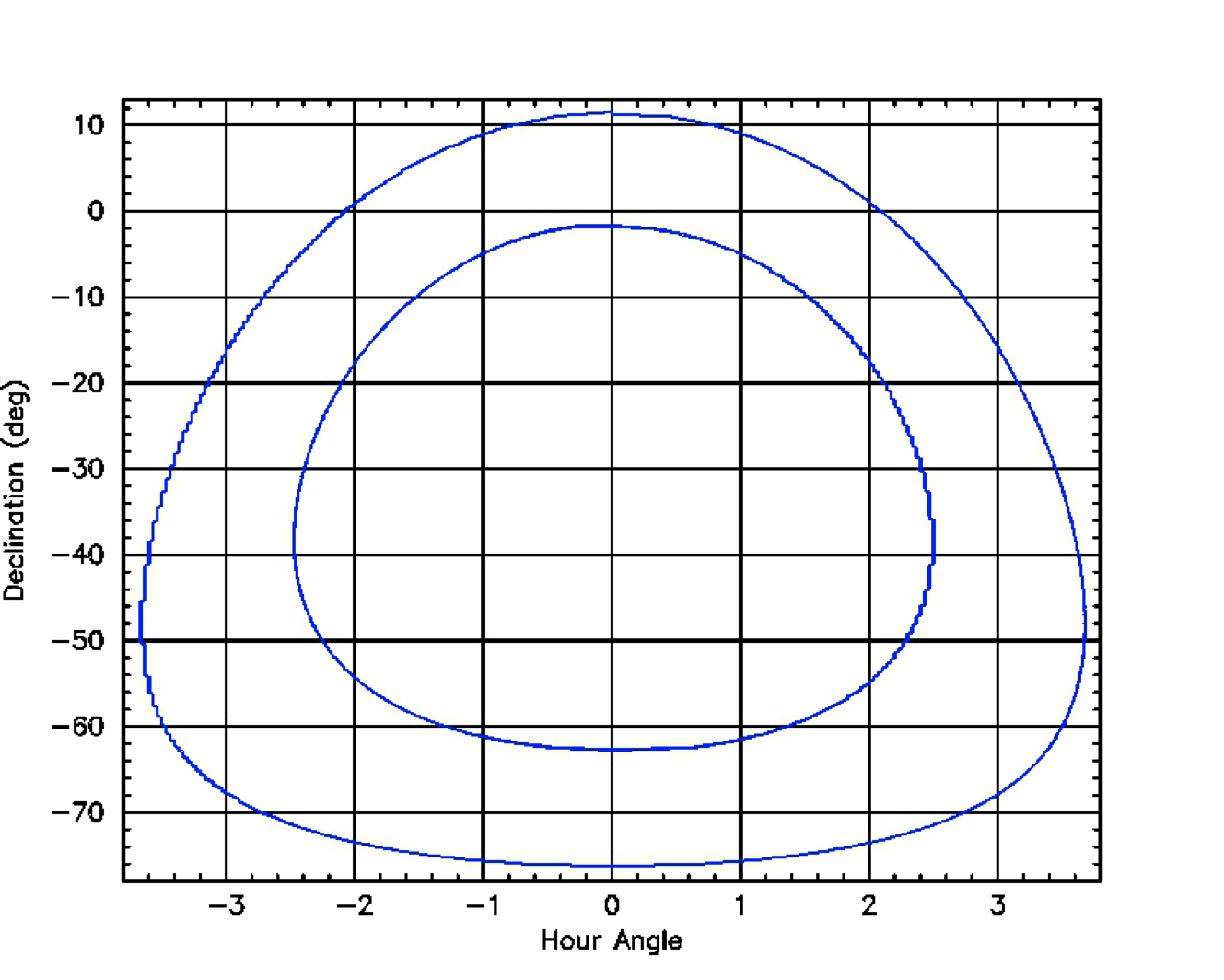
Figure 1: The visibility annulus of objects observable with SALT
The total maximum observing time, or visibility, for a celestial target is defined as the time it takes to transit the annulus, which is dependent on the Declination. However, the total maximum track time for an object, without having to move the telescope structure and re-acquire it, is determined by the tracker motion limits and is, therefore, equal to or shorter than the visibility time.
PIs should especially be aware that although Figure 1 and the Visibility Calculator may imply a total observing time of some hours, the tracker limits will necessarily curtail the maximum uninterrupted observing time available for a target. It is this maximum track time that defines the maximum length of an observing block.
Figure 2 shows the “actual” total maximum track time for objects as a function of Declination. For some Declinations (in the South and North), it is possible to re-acquire an object by stepping the telescope in azimuth, thereby extending the total observing time on a given night, as shown in the last graph. However, doing so incurs all of the normal overheads of repositioning the telescope and acquiring a target. Therefore, block times must be limited to available track times and observing time extended by multiple block visits.
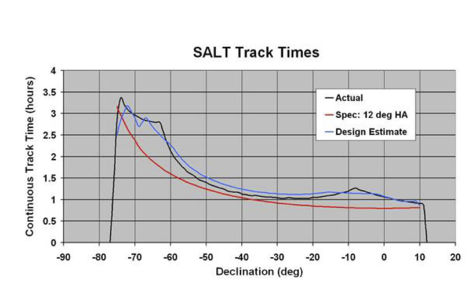
Figure 2: While objects can be visible for many hours continuously, a single track time may be shorter. At certain Declinations one is able to re-point the telescope in azimuth to continue for another track during the same visibility.
On the Visibility Calculator the track times can be seen by clicking at any location of the visibility curve or, even more useful, by viewing the new plot of track time vs time for a given target on a given night. The Visibility Calculator is available from the SALT Observing Tool webpage at:
http://salt4scientist.salt.ac.za/simulators-and-other-tools/
As part of the SALT design, the pupil moves during the track and exposures, thereby constantly changing the effective area of the telescope. Because of this, accurate absolute photometry and spectrophotometry are not feasible. Photometric calibration of imaging must be done using external data of the same field, though internal colour information can be obtained using filter cycles in the case of short exposures. Spectrophotometric standards are routinely taken and can be used for relative spectral (shape) calibration, but not absolute flux calibration.
All SALT observations are executed using Observing Blocks. These will be defined in detail in Phase 2, but it is necessary to be aware of the basic principles when planning observations for Phase 1.
Blocks are defined as the minimum schedule-able unit. A block must be allocated to a single priority and have a single Moon brightness, seeing range, and transparency specification.
For this semester, a block will consist of only:
a. one target
b. one acquisition
c. one or more science procedures or instrument configurations.
This sequence of observations plus overheads must fit within the target’s maximum available track time and must be at least 900 seconds long, inclusive of overheads (canonical overhead is 900 seconds for MOS and 600 seconds for any other instrument mode). Be aware that a target’s track time is less than or equal to its visibility time. For example, equatorial targets are visible for long periods of time (up to several hours), but they can only be tracked for about one hour or less at a time. Additional observing time is accrued by multiple block visits. To aid with the distinction between track time and visibility time and to help PIs with planning their observations, the SALT visibility calculator (see section 2.4) now includes a plot of track time vs time for a given object on a given night.
A block will be executed under the specified weather conditions. If the weather conditions change within the hour, the block will be repeated. After an hour, however, the block will be accepted regardless.
A block will also be repeated if the data quality was compromised by technical difficulties with the telescope or instrument.
Note that acquisition images are provided solely as a means of field identification and to allow positioning of the target(s). Acquisitions may thus be out of focus or otherwise unpalatable-looking: track time is valuable, and we do not want to waste time tweaking the acquisition images. The image quality is refined before science data are taken.
All investigators (PI and Co-Is) on a SALT proposal must have an account on the SALT server before the proposal can be submitted. This can be created by means of the Web Manager by pointing a browser to https://www.salt.ac.za/wm/Register/. After a successful registration, a confirmation email is sent, which includes instructions for validating the chosen email address. This validation is necessary before a proposal can be submitted with the investigator.
Once an account has been created, the Web Manager (https://www.salt.ac.za/wm/) can be used to view one's proposals and to update one's contact details. The home page of the Web Manager also provides links for downloading the latest version of the Principal Investigator Proposal Tool (PIPT).
All proposals are created and submitted with the PIPT, both for Phase 1 and 2. This is a stand-alone application requiring Java 1.6 or higher. While the Open JDK may work, using the Java environment provided by Oracle (http://www.oracle.com/technetwork/java/index.html) is strongly recommended. The PIPT itself can be downloaded from https://www.salt.ac.za/wm/.
New proposals can be created with the File > New Proposal menu item. The PIPT will ask whether the new proposal shall be a science or commissioning one. It is absolutely crucial to choose the science option, as otherwise the proposal won't be forwarded to the TAC and no time will be allocated to it.
As outlined in the next section, in addition to some general information, investigators, targets and instrument configurations have to be defined for a Phase 1 proposal. These may be added by right-clicking on a node in the navigation tree. Similarly, adding and removing content from a table can be accomplished by right-clicking on the table.
Warnings should be taken very seriously, as they often indicate a serious flaw in the proposal. In most cases, submission is only possible once the problem has been fixed. An explanation is displayed by clicking on the little warning sign next to the problematic input.
Before a proposal is submitted, it should be validated with the menu item Proposal > Validate. If the validation fails, this usually means that some required input is missing.
After the first successful submission of a proposal, a confirmation email with the proposal code is sent to all investigators. This proposal code uniquely identifies the proposal, and it should be quoted in the subject line of any email query related to the proposal. The proposal code is also added to the proposal itself, so that resubmissions do not generate new proposals in the database. It is a good idea to double-check that the correct proposal code is shown in a submitted proposal. No confirmation emails are sent for resubmissions.
When logging in to the Web Manager, a list of the user's proposals is shown. Clicking on any of the proposals leads to a page with the proposal details, which may be used to check a submitted or resubmitted proposal. However, it may take a few minutes before the content is fully visible (especially finding charts).
In addition to the the Web Manager, the PIPT and the Visibility Calculator, Simulator Tools are supplied for Salticam and RSS, which can be used to plan the required instrument setup and the necessary exposure time. They can be downloaded from http://salt4scientist.salt.ac.za/simulators-and-other-tools/ and as the other tools they require Java 1.6.
Both Simulators allow the user to define a target spectrum and an instrument configuration, and to calculate the signal-to-noise ratio expected for these. It should be noted that the Simulators do not take any overheads into account.
The Simulators have been verified for the current telescope and instrument throughput. However, the PIs should be aware that the wavelength ranges predicted by the RSS Simulator currently may have inaccuracies up to +/- 2 nm.
Proposals may be submitted, edited, and re-submitted at any time before the deadline, as many times as needed, until a final flag is set within the PIPT or in the Web Manager (WM). After the deadline edits are no longer possible.
Any questions during the submission phase should be emailed to salthelp@salt.ac.za. Previous submissions will have been assigned a program code - in that case, that code should be provided in the subject line.
The PIPT is deployed in various file formats, and the start page of the WM contains a brief description of how to install and launch it. The main items that need to be entered in the PIPT are:
All but the last two bullet points are entered in the respective boxes in the PIPT form, while the last two items must be included in the form as a PDF. This PDF is limited to four pages in length. The PDF must be generated using one of the templates provided (in Word, OpenOffice, or LaTex format). These can be downloaded from the Phase-1 instructions page at:
http://salt4scientist.salt.ac.za/phase-i/
Additionally, the latest versions of the RSS and SALTICAM simulator tools must be used to plan observations. These can be accessed from the SALT website:
http://salt4scientist.salt.ac.za/simulators-and-other-tools/
As stated in the previous section, please note that the Simulators do not take any overheads into account.
Simulated setups can be saved from the Simulator Tools, and these saved setups should be attached to a Phase 1 proposal in the PIPT for use in the technical reviews. The technical justification may refer to these attached instrument setups.
All Phase 1 proposals will first be directed to the SALT Astronomy Operations team for a technical feasibility assessment. Comments on technical feasibility will be forwarded to the individual TACs of the SALT consortium by 15 August 2013. The TACs will then allocate time to successful proposals in various priority classes and Moon brightness. The minimum time allocation for a successful proposal will be 900s per priority per Moon brightness.
The full TAC review and time allocation process is expected to end by 8 September 2013 and PIs will be informed of the outcome by the 15 September 2013. This will be followed by a Phase 2 submission period, during which the detailed observing Blocks will have to be submitted by the PIs to SALT operations using the PIPT. The strict deadline for the Phase 2 submission phase is 18 October 2013 with the new Semester observations commencing 1 November 2013. Please note that this Phase 2 proposal deadline will be strictly enforced, and no late proposals will be observed. This is crucial for planning the schedule for the semester. Proposals with Phase 2 material in before the end of the current period may also be considered for observations even before November 1, depending on the status of the queue of 2013-1 projects.
If there are co-investigators from multiple partners in a single proposal, it is up to the Co-Is to divide the proposed time between the relevant partners, or request all of it from one partner. If a program applies for time from more than one partner, all the relevant TACs will receive the application and will allocate their time individually.
In cases where only a small fraction of the time requested for a multi-partner partner proposal is awarded by the relevant TACs, then the SALT Astronomy Operations Manager will engage with the relevant TAC Chairs to ensure that the allocation can actually result in a meaningful program.
Detailed instructions on how to prepare the Phase 1 material are included within the Word/Latex templates and in the PIPT manual, which can be downloaded from:
https://www.salt.ac.za/wm/pipt_manager/PiptTutorial-3.0.pdf
Some common questions and issues are addressed below; however, a more complete, live, and frequently updated online FAQ is available at:
http://salt4scientist.salt.ac.za/phase-i-faq/
The SALT definition and break-down of sky conditions is as follows:
Dark (50% of time): Lunar phase angle > 135º (illuminated Lunar fraction of < 15% or Moon below horizon).
Gray (25% of time): Lunar phase angle 45º -- 135º (illuminated Lunar fraction = 15% -- 85%)
Bright (25 % of time): Lunar phase angle 0º -- 45º (illuminated Lunar fraction > 85%)
In Phase 2, there will be an opportunity to select more detailed lunar criteria (ie illuminated Lunar fraction) and angular Lunar distance. Please note that we have also introduced in the PIPT a default minimum angular Lunar distance of 30 degrees, which of course can be changed if necessary.
PIs with equatorial targets requesting Bright time please note that the Moon will likely be too close to the target for roughly ~50% of bright time.
Ideally all partners should attempt to distribute their observing time allocations accordingly. The instrument simulators should also be used to ensure that overly demanding observing conditions are not requested unnecessarily.
The standard measure of atmospheric turbulence is the Fried parameter, r0. The SAAO site uses an automated Differential Image Motion Monitor (DIMM) to measure this routinely and continuously. The blurring of an image at the focal plane of a large telescope, what we refer to as “seeing”, is derived from r0 using the standard model of atmospheric turbulence. It is a function of wavelength (λ) and airmass and the DIMM reports seeing using the convention of λ = 500 nm (essentially V-band) and airmass = 1.0. This is the value that is used to define observing conditions and make scheduling decisions.
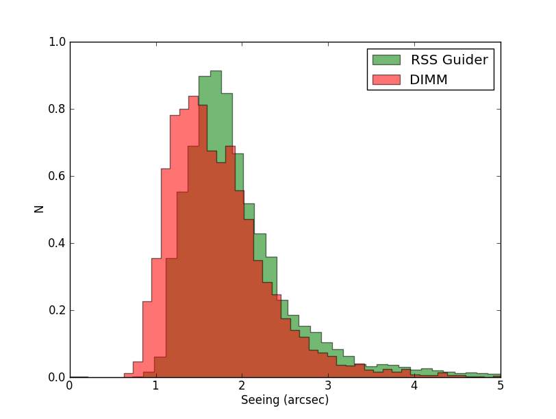
Figure 3: Seeing histograms from the SAAO DIMM and the RSS guider. The data are corrected to the middle of the visibility strip and taken from the same period of time, September through November 2011. This shows a factor of about 1.2 degradation between the intrinsic DIMM seeing and the IQ delivered to the SALT focal plane.
However, this zenithal seeing is not the same as the delivered image quality (IQ) at the SALT focal plane. The SALT visibility strip lies between 1.16 and 1.37 airmasses which leads to a factor of 1.1 to 1.2 degradation of seeing on average. There is also variable degradation in IQ due to SALT itself. Figure 3 shows histograms of seeing measured by the DIMM and the RSS guider corrected to the middle of the visibility strip. The median seeing reported by the DIMM is 1.5” versus 1.8” for the RSS guider. Proposers should be aware that 1” seeing equates on average to an IQ of 1.3-1.4” and that 1” seeing does not happen nearly as often as earlier site studies had found.
The following table indicates the expected best image quality performance of SALT (in terms of the FWHM and enclosed energy diameters (50% and 80%) of the PSF for different DIMM seeing values (all V-band). The PSF is basically described by a modified Moffat function.
DIMM zenith seeing | Seeing at average telescope airmass | FWHM | EE50 | EE80 |
1.0” | 1.2” | 1.4” | 1.6” | 2.6” |
1.5” | 1.7” | 1.8” | 2.0” | 3.3” |
2.0” | 2.3” | 2.4” | 2.7” | 4.2” |
These values are for a perfectly aligned primary mirror, which is currently not always the situation in the absence of closed-loop active control (e.g. because of the current lack of edge sensors) and remaining second order IQ issues associated with the primary mirror alignment. For these reasons, PIs should be aware that the above numbers cannot be guaranteed.
The statistics from the SAAO DIMM in Sutherland have been compiled for the last two semesters and are shown here in the next two figures (Figs 4 and 5). We believe these two figures clearly highlight that relaxing the seeing is one of the most efficient ways of increasing the likelihood of a block being observed. There is also a very clear difference in seeing conditions between the 2011-3 and the 2012-1 semesters. The 2011-3 semester had a median seeing of 1.38” while the median seeing was 1.66” in 2012-1.
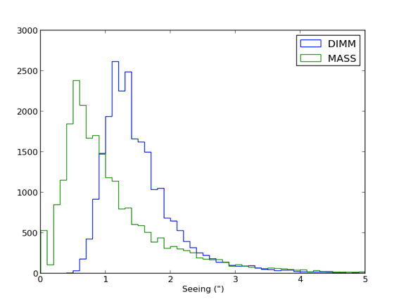
Figure 4 - Seeing histogram from our DIMM for the 2011-3 semester (1 Nov 2011 - 30 April 2012). The y-axis indicates the number of hours at that given seeing. The MASS seeing gives the seeing measurement from the free atmosphere (>1 km).
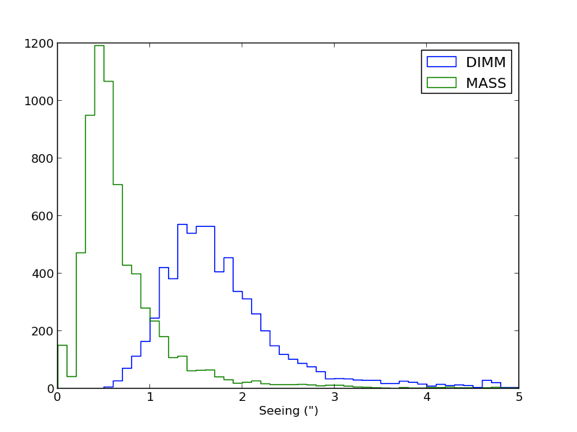
Figure 5 - Seeing histogram from our DIMM for the 2012-1 semester (1 May 2012 - 31 Oct 2012). The y-axis indicates the number of hours at that given seeing. The MASS seeing gives the seeing measurement from the free atmosphere (>1 km).
There are two types of SALT targets:
The previous section explained the basic concepts to understand when planning SALT observations, especially regarding the track times, the visibility of objects and the effect of the moving pupil for absolute (spectro)photometry. More detailed information on telescope performance and constraints on observations can be found at:
http://www.salt.ac.za/telescope/performance-characteristics/
http://www.salt.ac.za/proposing/observing-constraints/
Issues specifically affecting current Phase 1 proposal planning include:
The severe IQ issues that affected early SALT observations are now fixed. However, there is still about a factor of 1.2 degradation in IQ compared to intrinsic DIMM seeing as shown in Figure 3. The limiting factor in SALT’s IQ is largely the quality of the primary mirror alignment. We do not have active control of the mirror segments so alignment is only done periodically. They are done routinely during evening twilight and then during the night as needed. Observations must be interrupted to perform an alignment.
There is strong vignetting of the field-of-view, as shown in Fig. 6. Objects observed more than 2 arcmin from the centre of the field receive up to 10% less light, and this needs to be taken into account when planning to make use of targets over the full field of view. These numbers are greater than the specification and are currently under investigation.
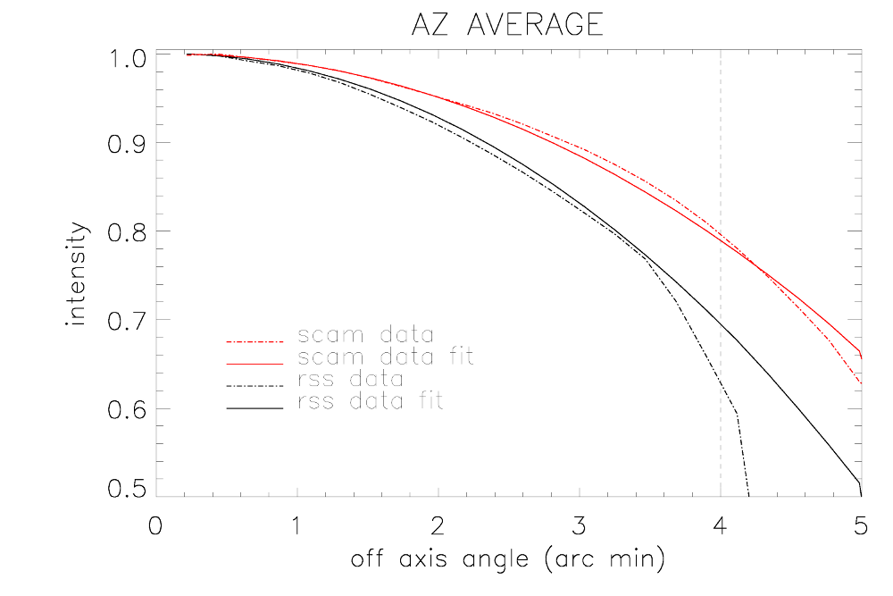
Figure 6. Vignetting of the FOV with RSS and SALTICAM.
There was a concentrated effort to recoat the whole primary mirror during 2012, and indeed this was achieved by October 2012. In addition, the primary is kept clean by regular (every week or two) cleaning with high-pressure CO2, and individual segments are normally taken out for washing and re-coating in a cycle of nominally about 12 months. The effect of not taking care of the primary is illustrated by the historical 2006-2008 throughput values of the mirror in Figure 7. Throughput of the telescope is routinely monitored using SALTICAM (since there are no significant optics in this instrument these values can be thought of as an approximation of the Telescope throughput). The nominal expected curve, as well as the system spec, can be compared against measurements derived from standard star observations and corrected for the estimated total efficiency of the instrument (filters, CCD, and foreoptics) and the atmosphere.
Figure 7 also shows the measured throughput situation from May 2012. After that, and during the time the bulk of the mirror was actually re-coated, Salticam was unfortunately not available for direct throughput measurements. An estimate was nevertheless made by comparing measurements done with RSS in late 2011 and May 2012, to measurements in September 2012. These indicate an overall improvement of ~15%, shown by the solid black curve.
The current situation appears to be close to expected in the red wavelength range, but falling short of expectations in the blue end. The reason for this is not certain, but a throughput shortfall in the SAC is suspected.
Since the RSS-derived estimate for current telescope throughput is not significantly different than what was used in the Simulators for the Period 2012-2, we have decided to not change the values for now, i.e. the measured 2012 values are still used. The RSS instrument specific throughput, with its significantly reduced blue sensitivity has also remained the same, and will remain so until an optical fix is undertaken (planned, but not yet scheduled). The “Fudge factor” curves in the right panel of Fig. 7 show the approximate factors, used by the Simulators, by which a totally nominal SALT is underperforming as a function of wavelength due to these throughput problems. SALTICAM is only affected by the “Telescope” curve, while RSS is affected by the product of the “RSS” and “Telescope” curves.
We stress that the current throughput values as discussed above are incorporated into the latest instrument Simulators which should be used for planning of 2013-2 programs. If changes become necessary, we will inform the community. Finally, note that while the atmosphere is corrected out from Fig. 7, its effect is included in Simulator tools and can be adjusted therein.
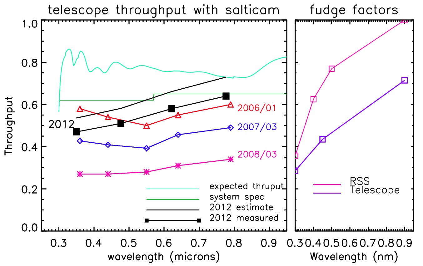
Figure 7. Current and historical telescope throughput values are shown at left compared to nominal values. The efficiency shortfalls comparing to nominal values, and incorporated in the instrument Simulators for the upcoming proposal round in 2013, are shown in the right panel separately for telescope and RSS-only. The latter is affected by the telescope as well. See text for more details.
The nominal collecting area of the primary mirror with a central track is ~55 m2, decreasing to ~40 m2 for extreme off axis tracker position. This means that SALT is equivalent to between a ~7 to 8 m diameter conventional telescope.
The current default collecting area in the instrument Simulators is set to 46 m2 (or approximately 53 fully illuminated segments) – this corresponds to experimentally derived averages of visible pupil area with tracker obscuration over a full track, and also makes allowance for the fact that the throughput calculations referred to above are normally done for a dozen or so best-quality segments. The collecting area is an adjustable parameter in the Simulators, but it should only be changed with caution.
All of the latest news about the SALT calibration plan could be found at:
http://www.salt.ac.za/observing/proposing-for-salt-observations/salt-calibration-plan/
SALT calibration data are divided into four categories:
Please see section 6.7 for the current semester SALTICAM calibration plan and section 7.8.2 for the corresponding RSS calibrations. No calibrations are needed for BVIT.
SALTICAM is a UV-Visible (320 - 900 nm) imaging and acquisition camera, capable of high time resolution imaging (at ~10 Hz). It consists of two E2V 44-82 CCDs (2048 x 4102 x 15 µm pixels), which are physically separated by a 1.5 mm gap and are read out by four amplifiers. SALTICAM is at prime focus; however, it is fed by a fold mirror and has a reduced focal ratio of f/2. The result is a nearly 10-arcmin diameter field of view, with the central 8-arcmin diameter portion being used for science and the outer annulus for guide stars. The plate scale is 0.14 arcsec/pixel. Basic information required for observing is provided in this section.
There are four possible combinations for readout speed and gain settings, returning gain values between 1.0 and 4.5 electrons/ADU with readout noise of either 3.3 or 5 electrons per pixel (Table 1; Table 2). The dark current is typically less than 1 electron per pixel per hour. Full well depth is on the order of 170k electrons. Pixel prebinning from 1x1 to 9x9 (independent in each direction) and up to ten subframe windows can be selected. The readout times for full frame, 2x2 binning are given in Table 2. A wide range of filters are available, spanning the wavelength range 320-950 nm (Section 6.4; Table 4).
Readout Setting | Gain Setting | Actual e/ADU |
Fast | Faint | 1.55 |
Fast | Bright | 4.5 |
Slow | Faint | 1.0 |
Slow | Bright | 2.5 |
Table 1: Gains for the four different readout modes selectable on SALTICAM
Detector Mode | Pre-bin | RO mode | RO Noise (e-/pix) | Total Readout Time (sec)* |
Full Frame | 2x2 | Slow | 3.3 | 21 |
Full Frame | 2x2 | Fast | 5.0 | 14 |
Table 2: Readout (RO) times of SALTICAM for the 2x2 binning. Refer to the SALTICAM web-pages and PIPT for times of other binnings. *Inclusive of CCD readout, disk writes, and software overheads.
Standard modes of operation are normal imaging (full-frame readout), frame transfer (half-frame readout), and slot mode (144-row readout). Specific characteristics for these modes, as well as the specialised modes of non-sidereal tracking and drift scanning, are discussed below. Note that absolute photometry is not possible with SALTICAM alone because of the moving pupil.
More details on this instrument can be found at in Section 12.1, the first Appendix to this document. A simulator that uses target characteristics and a detector configuration to return count rates, signal-to-noise ratios, pixel saturation, and readout times can be downloaded from the following website: http://salt4scientist.salt.ac.za/simulators-and-other-tools/.
SALTICAM is available for the 2013-2. There is a new website that lists the currently installed SALTICAM filters: http://salt4scientist.salt.ac.za/telescope-status/.
Though guiding with SALTICAM is possible, it has several features redering it not useful for many applications (see Section 6.6). Overall, we suggest limiting SALTICAM exposure times to approximately 120 seconds with open-loop tracking.
Normal imaging is the basic, full-frame SALTICAM mode, which also serves as the acquisition mode for spectroscopic observations. The sub-framing, preamplifier binning, gain, and filter options listed above are available.
The frame transfer mode ensures moderate time resolution (a few sec) and no dead time. In frame transfer mode, a mask covers the lower half the detector (both chips). At the end of each exposure, the image in the top half of the chip is rapidly (0.2 sec) shifted to the lower half where it is read out while the next image in the top half accumulates during the next exposure, thereby ensuring no dead time.
A list of the minimum exposure times for frame transfer mode in each binning is provided in the third column of Table 3.
Slot mode ensures high time resolution (to 0.05 sec) with practically no dead time. It only works with the FAST readout speed. In this mode, a mask is advanced over the entire detector except for a horizontal slot of 20 arcsec height just above the frame-transfer boundary. At the end of each exposure, 144 rows are moved down and this allows exposure times as short as 0.05 sec. Timing tests carried out with an independent GPS demonstrate that the absolute and relative timing accuracy of slot mode are good to a few tens of millisec.
The minimum exposure time for slot mode in each binning setting is provided in the second column of Table 3. More information on slot mode is available in Appendix section 12.1.
Please note that the position angle is a critical parameter for most slot mode observations in order to image both the target and a comparison. Finder charts should clearly indicate the position angle and the location of the slot (which is done automatically by the SALT finder chart tool http://pysalt.salt.ac.za/finder_chart/).
Pre-binning | Slot Mode (sec) | Frame Transfer (sec) |
1x1 | 0.70 | 15.90 |
2x2 | 0.30 | 4.70 |
3x3 | 0.20 | 2.80 |
4x4 | 0.15 | 2.00 |
5x5 | N/A | 1.70 |
6x6 | 0.08 | 1.40 |
7x7 | N/A | 1.30 |
8x8 | 0.07 | 1.10 |
9x9 | 0.05 | 1.10 |
Table 3: Minimum exposure times per binning for SALTICAM Slot Mode and Frame Transfer.
For imaging objects in the solar system, non-sidereal telescope tracking might be preferred. Initial tests of the implementation and accuracy of this mode at slow (a few arcsec per hour) and fast (hundreds of arcsec per hour) rates have been carried out. Initial analyses indicate that the telescope seems to be correctly interpolating ephemerides in order to point and then tracking at the correct nonsidereal rates; however, we have not yet quantified any errors on the pointing and tracking. Any non-sidereal tracking proposals are considered shared risk.
Drift scanning is an imaging mode where the telescope is parked at a stationary position and the CCD readout is clocked at the sidereal rate. This can be used to produce long imaging “strips” on the sky, e.g. for surveys. While some preliminary SALTICAM drift scanning tests have been successfully completed, there are still some issues to iron out before this mode is offered to the community. Therefore, it will not be available for this proposal period.
All SALTICAM sensitivity calculations for planning observations should be done with the newest version of the SALTICAM Simulator (http://salt4scientist.salt.ac.za/simulators-and-other-tools/). These numbers are based on throughput tests with a burst mirror, as well as Sloan comparison fields, and have been extrapolated for a typical pupil during a track.
The count rates and signal-to-noise ratio numbers can be extrapolated to other exposure times and fainter/brighter targets. We have directly verified count rates up to about 5-minute exposures and these behave as expected. Longer integrations are not practical due to the difficulties with auto-guiding (see Section 6.6) and SALT’s current open-loop tracking performance. Thus, the deepest SALTICAM exposures should ideally be constructed from dithered and co-added ~2 minute exposures. Whether the ideally scaled signal-to-noise ratio is reached depends on e.g. the quality of flat-fields (see Section 6.7.2) and the stability of the PSF of sources over tens of minutes (c.f. the current lack of active segment alignment). Therefore, we urge the PIs to be conservative in estimates of deep SALTICAM imaging until proper characterisation has been obtained. We do not yet have demonstrated sensitivity performance values for longer stacked sequences, though we will update these values and inform the community if such results become available during the course of the current period.
SALTICAM has an eight-position filter magazine. Available filters are listed in Table 4. Filter transmission data are provided for a collimated beam at the links under ”Filters” at http://www.salt.ac.za/telescope/instrumentation/salticam/specifications/.
The SALTICAM CCDs were optimised for visible and near UV imaging, thus no effort was made to minimise fringing at near IR wavelengths. We have not yet quantified the amplitude of fringing in all filters. We have observed fringes with an amplitude of ∼10% peak-to-trough for red, narrow-band filters such as z’. Fringing is not an issue for broadband filters or those at the shorter end of the wavelength range.
Type | Name |
Johnson-Cousins | U, B, V, R, I |
Sloan | u’, g’, r’, i’, z’ |
Strömgren | u, b, v, y, H-β wide, H-β narrow, SRE1, SRE2, SRE3, SRE4, Clear |
Other | H-α (zero redshift) 380-nm (FWHM 40Å) neutral density |
Table 4: SALTICAM filters
As stated above, due to the flat-fielding difficulties as a result of the moving pupil, it appears that best photometric results over the field of view will be obtained with dithered observations.
The most productive dithering schemes will depend on the science goal and size of science targets. For Phase 2, a user-selectable dithering pattern is supported in the PIPT. Please note, however, that SALT does not provide automatic dithering which makes such observations manual and slightly time consuming. Dithering will affect overheads, since every offset will take approximately 15 seconds. Note that the dithering step size is not restricted, but there is a risk of losing the guide star if the step size is large -- however see Section 6.6 below for the sensibility of even using guiding. If guiding is nevertheless desired, we thus recommend the total dithering pattern to be constrained within approximately one square arcminute -- if larger steps are required, please note to the observer to select a central guide star.
While SALTICAM is equipped with an auto-guider, it has several serious design limitations that greatly degrade its overall usefulness:
Because of these shortcomings we do not advocate the use of the SALTICAM auto-guider during normal imaging. SALTICAM has low read-noise so the sky limit is reached quickly in most broadband filters. It’s reached in under a minute for even U, u′, and H-α. Our current open-loop tracking performance allows unguided exposures of up to 2 minutes which is sufficient for all but the bluest Strömgren filters. Work to improve our open-loop tracking is on-going.
We do support using the auto-guider during slot and frame-transfer mode observations. However, it is not commonly used due to the extra overhead involved in configuring it for a field and therefore it must be specifically requested.
Please refer to section 5 for a general description of SALT calibrations.
Our current SALTICAM calibrations plan (section 6.7.2) is based on the specifications of the SALT telescope and our current experience. We would like to highlight the following:
For all the reasons stated above, the current SALTICAM calibrations plan for this semester is:
Please note that a larger number of calibrations will need to be justified and we cannot guarantee that these calibrations will be useful.
The Robert Stobie Spectrograph (RSS) is the main work-horse instrument on SALT and is a complex multi-mode instrument. This means it has a wide range of capabilities -- excellent for astronomers, but a nightmare for the engineers who built it, are commissioning it, and maintain it!
RSS resides at prime focus, where it takes advantage of direct access to the focal plane, and was designed to have a range of capabilities and observing modes, each one remotely and rapidly reconfigurable. In keeping with the overall philosophy of exploiting those areas where SALT has a competitive edge, the instrument has several unique, or rare, capabilities. These capabilities include the following:
Currently RSS is routinely being used for the following modes:
Commissioning will be continued in the near future for the polarimetry and dual-etalon Fabry-Perot modes (currently stalled). For current sensitivity and throughput issues refer to Sections 4.3 and 7.5, and Figure 7.
7.2 Gratings
RSS has a complement of six transmission gratings: one standard surface-relief grating and five volume phase holographic (VPH) — see Table 5. VPH gratings have the characteristic that their efficiency varies with input angle (see Fig. 8), and thus a single grating can cover a large wavelength range with good efficiency by changing the relative angle between the collimated beam and the grating normal. This is accomplished using a rotating stage. The RSS camera is then articulated to twice the grating angle since the VPH efficiency curve for a given grating angle typically is at a maximum at the Littrow wavelength. The angle of the grating also affects spectral resolution. The higher the value of the grating tilt, the higher the spectral resolving power for a given slit width. The RSS Simulator tool found at:
http://salt4scientist.salt.ac.za/simulators-and-other-tools/
should be used to determine the optimal grating angle and slit-width for an observation. Note also that a feature of VPH gratings is that the resolution and wavelength range of an object depends on the distance of the target from the optical axis. While this is not an issue for long-slit spectroscopy, it will affect multi-object spectroscopy (see Section 7.4.4 for more details).
Grating Name | Wavelength Coverage (nm) | Usable Angles (deg) | Bandpass per tilt (nm) | Resolving Power (1.25” slit) |
PG0300 | 370-900 | 390/440 | 250--600 | |
PG0900 | 320-900 | 12-20 | ~300 | 600-2000 |
PG1300 | 390-900 | 19-32 | ~200 | 1000-3200 |
PG1800 | 450-900 | 28.5-50 | 150-100 | 2000-5500 |
PG2300 | 380-700 | 30.5-50 | 100-80 | 2200-5500 |
PG3000 | 320-540 | 32-50 | 80-60 | 2200-5500 |
Table 5: RSS grating complement
All gratings are used in first order only. Second-order contamination is removed through the use of order-blocking filters.
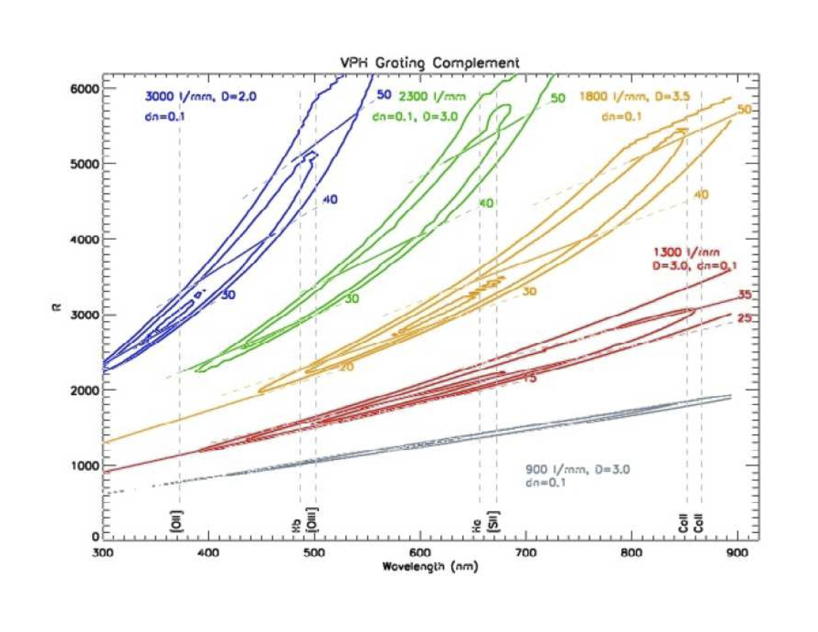
Figure 8: VPH grating efficiency as calculated using Rigorous Coupled Wave (RCW) analysis in resolving power versus wavelength for a 1.5” slit. The contours correspond to 90%, 70%, and 50%. Wavelength coverage for a few angles is shown for each grating.
Five order-blocking filters are available for RSS spectroscopy: one clear, three UV blocking, and one blue blocking. These filters are listed in Table 6. There are also 40 interference filters to be used with Fabry-Perot observations as well as narrow-band imaging (Table 7). All filter transmission curves are available online at:
Type | Name |
Clear | PC00000 |
UV | PC03200, PC03400, PC03850 |
Blue | PC04600 |
Table 6: RSS order blocking filters
The RSS optical design is not optimized for broad-band imaging. Narrow-band imaging may be performed with any of the 40 Fabry-Perot interference filters listed in Table 7.
There is considerable fringing in the red narrow-band filters when they are illuminated at discrete wavelengths. Fringing has only been measured in the few filters mounted to date that are long-ward of 750 nm. In all filters tested, fringing is negligible for broadband illumination (sky and QTH lamps) with peak-to-trough variations of 2%. With arc lamp illumination (Ne or ThAr), the PI07500 filter shows no fringing while the PI08350, PI08535, and PI08730 filters have obvious fringing at levels of 10-20% peak-to-trough.
RSS imaging can be done in FT and slot modes; however, the throughput of SALTICAM is higher, making it the preferred instrument for such observations. Timing tests carried out with an independent GPS demonstrate that the absolute and relative timing accuracy of RSS slot mode are good to a few tens of millisec.
The SALT RSS Fabry-Perot system provides spectroscopic imaging over the whole RSS science field of view (8 arcmin diameter) in the wavelength range 430-860 nm with spectral resolutions ranging from 300-10000 depending on the mode used and wavelength observed.
The system consists of three etalons with gap spacings of ~0.6 nm, ~2.8 nm, and ~13.6 nm. The etalons are referred to as the low resolution (LR), medium resolution (MR), and high resolution (HR) etalons, respectively. The LR etalon can be used in its normal LR mode or configured as an even lower resolution tunable filter (TF). The MR and HR etalons are normally used in conjunction with the LR etalon in LR mode
However, during commissioning of the dual-etalon modes, a serious reflection problem between the two inserted etalons was discovered. Multiple reflections between the etalons introduces a series of ghost images and significantly degrades throughput. Rectification of this problem is underway, but may take several months to complete. In the interim, the original dual-etalon MR and HR modes are NOT available. However, single-etalon MR mode is available. Table 7 shows the filters that are available for use with Fabry-Perot.
Table 7: RSS Narrow-band (Fabry-Perot) Filters
Name Centre (Å) FWHM (Å)
pi04340 4349.4 79.1
pi04400 4412.3 92.4
pi04465 4478.1 84.9
pi04530 4530 90
pi04600 4600 95
pi04670 4670 100
pi04740 4760.2 111.1
pi04820 4820 105
pi04895 4912.5 105
pi04975 4990.6 107.5
pi05060 5071.5 110.5
pi05145 5152.1 109.2
pi05235 5237 119.1
pi05325 5325 125
pi05420 5420 130
pi05520 5520 135
pi05620 5631.5 137
pi05725 5731.1 133.6
pi05830 5833.6 142.8
pi05945 5946.5 164.1
pi06055 6062.2 148.6
pi06170 6178.8 169
pi06290 6300.2 158.3
pi06410 6418.4 161.5
pi06530 6535.5 156
pi06645 6647.4 148.8
pi06765 6765 167.5
pi06885 6894.3 181.8
pi07005 7020.8 162.1
pi07130 7131.3 140.4
pi07260 7252.7 184.1
pi07390 7400 218
pi07535 7555.6 200.8
pi07685 7691.9 168.9
pi07840 7831.6 207.6
pi08005 7999 249.2
pi08175 8175.1 225.2
pi08350 8350 245
pi08535 8535 260
pi08730 8730 275
As of June 2013 TF, LR, and single-etalon MR modes are all calibrated for use in the H-α region (650-690 nm). LR and MR are both calibrated in the H-β/[O III] region (480-510 nm) and MR is calibrated in the 820-870 nm region. We are also accepting proposals for wavelength regions that are not currently calibrated. Wavelength calibration is an ongoing process, however, and PIs should be aware that uncalibrated wavelength regions observations will only be conducted as time and resources allow.
Flexure within RSS significantly impacts Fabry-Perot calibration so Fabry-Perot observations must be carried out as close as possible to the parallactic angle. Specific positions angles cannot be requested for Fabry-Perot observations. Because the position angle of the parallactic angle can vary significantly along a track or between east and west tracks it is very difficult to predict the location of the CCD gaps a priori. To maintain maximum flexibility in scheduling we recommend that multiple dithered scans be obtained in cases where the object(s) of interest do not fall completely on the middle CCD.
All available Fabry-Perot modes need further work on flat-fielding, throughput determination, and stability characterisation in order to be considered fully commissioned and ready for routine science observations. Flat-fielding, in particular, has recently been discovered to be very problematic and work is actively ongoing to fully characterize this and how it might be calibrated properly. Therefore, all Fabry-Perot observations are still considered shared-risk in this call.
Notwithstanding the previous comments, the LR and single-etalon MR modes have been used successfully for several science programs. The TF mode has not yet been used for science observations, but is considered ready for use since it shares the same hardware as LR mode. Emission line programs such as H-α mapping are generally fine to pursue with the single-etalon MR mode. Absorption line studies may be more problematic. Observers should use the tables of etalon free spectral range given in the etalon technical reports and the blocking filter curves to estimate the effects on their particular program. Because of the small free spectral range of the HR etalon, single-etalon mode HR is regrettably not usable.
Further details and links to useful documentation can be found at the SALT Fabry-Perot web page: http://www.salt.ac.za/technical-info/instruments/rss/rss-fabry-perot/
Tables containing the FWHM of the spectral resolution, the resolution and free spectral range of each etalon as a function of wavelength are included in that webpage. This information is helpful for proposal planning. A detailed description of the system is given in the paper by Naseem Rangwala, Ted Williams and their collaborators available at: http://iopscience.iop.org/1538-3881/135/5/1825
Additionally, Ted Williams has produced an Introduction to Fabry-Perot on SALT: http://www.salt.ac.za/fileadmin/files/Technical_Info/Instruments/RSS/AnIntroductiontoFabry.pdf
Long-slit spectroscopy is the most commonly-used mode for RSS. The choice of slit widths is driven by considerations of resolution and throughput. A variety of slits is available to cover the range of atmospheric seeing conditions expected at the site. The RSS slitmask magazine has room for ten, tilted longslits. These allow for the SALT Imaging Camera (SALTICAM) to be used as a slit-viewing camera. Currently available slits are specified in Table 9.
# | Slit | Size |
1 | 0.6 | 0.60”x8’ |
2 | 1.0 | 1.00”x8’ |
3 | 1.25 | 1.25”x8’ |
4 | 1.5 | 1.50”x8’ |
5 | 2.0 | 2.00”x8’ |
6 | 3.0 | 3.00x8’ |
7 | 4.0 | 4.00”x8’ |
Table 9: Available long-slits for RSS
All available gratings are described in Section 7.2. All available order-blocking filters are described in Section 7.3.
Some commissioning data has been taken for long-slit spectra of non-sidereal targets. Tracking at the object rates is not commissioned. However, observations of bright targets whose motion is aligned along a wide slit (2” or greater) will be accepted. It is the responsibility of the PI to determine the correct PA to keep the target in the slit and to ensure that the target is bright enough to appear in the slit view images (so that the SA and SO can push it back into the slit if it moves out).
RSS has multi-object spectroscopy (MOS) capability. Slits are laser-cut on carbon-fibre masks in Cape Town. The instrument can hold 30 MOS masks in a magazine at any given time, and the rest of the fabricated masks also reside at the telescope.
The masks are manufactured following user specifications through a java-based RSS Slit-Mask Tool (RSMT). This tool is fully functional and is downloadable from the SALT proposal tools webpages:
http://salt4scientist.salt.ac.za/simulators-and-other-tools/
There is also work being done on an updated version of the RSMT with improved functionality to optimise mask designs from large source lists. Both will likely be supported for the 2013-2 Phase 2 stage.
No SALT pre-imaging is required for the mask preparation provided FITS files of the field containing astrometric solutions accurate enough for the PIs science goal are available. We stress that high-quality astrometric solutions in the PIs images are absolutely crucial for successful MOS observations. Pre-imaging can naturally be obtained with SALTICAM as well; however, these require their own Blocks which have to be observed well in advance of the MOS observations. Pre-existing astrometric files are strongly preferred and the reference stars for alignment and the science slits themselves must come from the same WCS source. MOS masks use 3-7 5”x5” holes for reference stars and alignment is done with feedback from through-slit images. Another important aspect to remember in the Phase 2 for MOS observations is the restricted Declination-dependent availability of field orientation; a document describing this can be found here:
http://www.salt.ac.za/fileadmin/files/observing/documents/SALT_PA_Visibility.pdf
One specific characteristic of VPH gratings used on RSS to keep in mind is that the wavelength dependence of the efficiency, as well as the simultaneous wavelength coverage for a given grating setup depends on the input angle to the grating. In MOS, the light entering through off-axis (in the dispersion direction) slits will hit the grating at different angles. Thus, the efficiency for the off-axis objects will be different than for the on-axis objects. This will in general not be symmetric either. Figure 9. illustrates this, and MOS users should consult the VPH grating simulator at http://www.sal.wisc.edu/PFIS/docs/rss-vis/ebb/pfis/observer/specsim.html
for details.
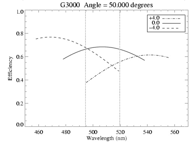
Figure 9. Example of the effect of blaze-angle on wavelength range and efficiency in MOS mode. Shown are the extreme cases of having an object at the edges of the RSS field-of-view, ±4’ off-axis.
While MOS commissioning as a whole is now completed and MOS projects are regularly observed, there are still issues being worked on, and telescope design features are placing restrictions on optimal MOS performance. An issue with no easy solution is that field rotation is open-loop on SALT by design. There is typically a 0.05 degree drift in rotation during a 30 min track around the guide star, which would, at the edge of a field correspond to a spatial drift of 0.4”. Experience has shown however that the rate is not constant, and can be more. An exception are very Southerly tracks where the rotation is at its smallest, and re-alignment is not necessary until at least 1h. For this reason we suggest the following:
Based on our first two periods of MOS observations the three most frequent issues we have seen when executing submitted programs are 1) the tendency of PIs to underestimate the required exposure times for faint targets, 2) insufficient accuracy in the WCS of the reference stars, and 3) some PIs specifying too short slits (<10”) which will make sky subtraction very difficult. A set of instructions for preparation of MOS Phase 2 material, including e.g. proper selection of reference stars, can be found from the Phase 2 FAQ page at
http://salt4scientist.salt.ac.za/phase-ii/
All polarimetric modes are currently unavailable due to problems with the Wollaston beamsplitter mosaic. No polarimetry proposals will be accepted in the current proposal call.
This mode of operation ensures moderate time resolution (a few sec) and no dead time.
In Frame Transfer mode a mask covers the lower half the detector (all three chips). At the end of each exposure, the image in the top half of the chip is rapidly (0.2 sec) shifted to the lower half where it is readout while the next image in the top half accumulates during the next exposure, thereby ensuring no dead-time.
A list of the minimum exposure times for frame transfer in each binning can be seen in the third column of Table 10.
Frame Transfer spectroscopy is only currently available with the 1.5” slit, but please contact the SALT team should you require a different width.
Pre-binning | Slot Mode (sec) | Frame Transfer (sec) |
1x1 | 0.70 | 20.0 |
2x2 | 0.30 | 8.4 |
3x3 | 0.20 | 4.7 |
4x4 | 0.15 | 2.0 |
5x5 | N/A | 2.6 |
6x6 | 0.08 | 2.2 |
7x7 | N/A | 1.9 |
8x8 | 0.07 | 1.7 |
9x9 | 0.05 | 1.6 |
Table 10: Minimum exposure times for Frame Transfer and Slot Mode for RSS.
All RSS sensitivity calculations for planning observations should be done with the newest version of the RSS Simulator. PIs are warned that the RSS throughput below 400 nm is not nearly as good as expected. See Section 4.3 and Figure 5. for more information. All current information on both the telescope and instrument throughput based on recent measurements is incorporated into the RSS Simulator.
However, we have noticed through experience that PIs still regularly underestimate the required exposure times, especially with fainter targets. Please be conservative when selecting the conditions for the simulation, and remember the IQ and seeing definitions (see Section 3.2.2) and that seeing and image quality (which is rarely perfect, as the simulation assumes) has a large effect on the S/N of targets fainter than sky brightness. In addition, be sure you understand different definitions of S/N, per pixel or per resolution element, and what these mean for your science.
As a guideline, approximate magnitude limits at a mid-range wavelength for each grating are tabulated in Table 11. The limits have been calculated for 30-min exposures using the 1.5” slit, with 1.3” seeing at Zenith, in dark conditions, for an A0V type star (point-source). The numbers are applicable to long-slit and MOS observations. The magnitude limit here corresponds to signal-to-noise ratio of 5 per pixel in 2x2 binning over a 2 x FWHM aperture spectral extraction at the tabulated wavelength. As a crude rule of thumb for limiting magnitudes in good conditions, verified by actual observations, V=23 magnitude point sources can produce “measurable flux” in ~30 minute exposures with the PG900 grating and V=21 magnitude point sources with the PG3000 grating in blue settings.
Grating | Central λ (nm) | Resolution (λ/δλ) | Mag Limit (V) |
PG0300 | 620 | 350 | 21.9 |
PG0900 | 605 | 1065 | 21.5 |
PG1300 | 665 | 1800 | 21.1 |
PG1800 | 677 | 2890 | 20.6 |
PG2300 | 566 | 3220 | 20.7 |
PG3000 | 434 | 3215 | 20.7 |
Table 11: Guideline RSS sensitivities in the middle of the ranges of the gratings. See Figure 6 for available ranges. The RSS Simulator tool should be used for more detailed calculations.
We also draw to the attention of RSS users that the current RSS Simulator has inaccuracies up to ~2 nm in its wavelength range predictions to be noted when assessing the locations of the CCD gaps and edges.
7.6 Guiding
The RSS auto-guider is routinely used for almost all RSS observations. Unfortunately, its sensitivity is limited to rather bright guide stars. The practical limit is V ~ 16 mag with 16.5 mag possible in good seeing. This is usually not a problem for long-slit work, but can be an issue for MOS and Fabry-Perot where the available field for selecting a guide star may be much more restricted.
The nominal closed-loop tracking performance with a bright guide star is about 0.2” RMS. With fainter guide stars and longer integrations this can degrade to 0.4” RMS. Work is ongoing to improve this and to improve the sensitivity of the guide camera.
The RSS autoguider focus functionality was not successful and is no longer available. Work is ongoing for alternative solutions, but at the time of writing, focusing the telescope is still a manual process and is expected to remain so for several months.
In principle, it should also be possible to use SALTICAM as a guide camera in conjunction with the pellicle (software guiding). The pellicle degrades throughput to RSS by ~5-7%, but this mode provides the ability to correct for drifts in field rotation, making the throughput loss potentially worthwhile. However, since the current pellicle also degrades the SALTICAM image quality significantly, guiding this way has not yet been successful. Plans are afoot for a new glass pellicle, but this is not expected to be available for 2013-1 semester.
Our positional repeatability is currently 0.3” RMS for step sizes < 1” while guiding and 0.5” RMS for step sizes > 1”, as measured by performing offsets of sizes varying from 0.5” to 30” and returning to the original position. This accuracy is not sufficient for reliable blind offsetting in most cases, so for faint objects we recommend providing a brighter alignment object and a PA that will ensure placement of the fainter object in the slit. The PA positioning accuracy is at least 0.5 deg, so finding a star of V=15-20 mag range at 60” distance would ensure the positioning of the slit with <0.5” accuracy. It is safer to use slit widths of 1.5” or more, and to use alignment stars as close as possible.
This lack of offset repeatability greatly curtails our ability to do accurate nodding. Couple this with the lack of software to support it, it means we will not be offering nod-and-shuffle as an observing mode during 2013-1.
All of the comments and caveats about SALTICAM dithering that are discussed in Section 6.5 apply to RSS as well. The accuracy of the dithering is, again, limited currently to 0.5” RMS. For some purposes (e.g. Fabry-Perot), this is perfectly fine. For others (e.g. dithering blindly between different slit positions), it may not be. However, since in most cases an object will be visible on the slit-viewer, the observer just would re-check alignment before re-starting exposures (60 sec overhead is defined for nodding along the slit, which includes the move and tweak of position if required).
The RSS calibration plan (see section 7.8.2) is based on the SALT telescope specifications and on current experience. We would like to point out the following items:
All calibrations should be requested by the relevant check-boxes in the Phase-2 PIPT. For overhead estimations without using the PIPT Table 12 in Section 10. can be used as well.
The calibration plan (see Section 5.1 for definitions) for RSS for the upcoming semester is:
Again, we do not recommend these and have not found them to be effective for calibrations.
The SALT HRS is a dual-beam (370-555 nm and 555-890 nm) fibre-fed, white-pupil, échelle spectrograph, employing VPH gratings as cross dispersers. The cameras are all-refractive. The concept is for SALT HRS to be an efficient single-object spectrograph using pairs of large (350 μm to 500 μm; 1.6-2.2 arcsec) diameter optical fibers, one for source (star) and one for background (sky). Some of these will feed image slicers before injection into the spectrograph, which will deliver resolving powers of R ~16,000 (unsliced 500 μm fibres), ~37,000 (sliced 500 μm fibres), and ~67,000 (sliced 350 μm fibres). A single 2k x 4k CCD will be sufficient to capture all the blue orders, while a 4k x 4k detector, using a fringe-suppressing deep-depletion CCD, will be used for the red camera. Complete free spectral ranges are covered by both the blue and red arms.
HRS construction began at Durham University’s Centre for Advanced Instrumentation in late-2007 and it is scheduled to begin science commissioning on the telescope in late September 2013. An Expression of Interest call was released on 1st July 2013 inviting submission of HRS science commissioning proposals. The initial re-assembly and commissioning is expected to take 4-6 weeks. These programs will be undertaken on a shared-risk basis and will not be charged to partners allocations. A modest amount of time (~50 hours in 2013-1 semester, and probably a similar amount in 2013-2) is being set aside for these programs.
As previously mentioned, SALT HRS offers four different operational modes, which vary in spectral resolution at the expense of instrument throughput. Table 12 summarizes the four modes along with their options.
Parameter | High Resolution Mode | Medium Resolution Mode | Low Resolution Mode | HS Mode |
Fibre Diameter (arcsec) | 1.56 | 2.23 | 2.23 | 1.56 |
Slit width (arcsecs) | 0.355 | 0.710 | 1.673 | 0.355 |
Image Slicers | 3 slices | 3 slices | No | 3 slices |
Blue arm resolution | 64400 | 36600 | 16200 | 64400 |
Red arm resolution | 69200 | 37300 | 16200 | 69200 |
Blue arm transmission (total %) at 450nm* | 2.8 | 3.0 | 6.8 | 1.7 |
Blue arm transmission (total %) at 750nm* | 4.2 | 4.5 | 9.8 | 2.5 |
Fibre mode scrambling | No | No | No | Yes, permanent |
Nod and shuffle | No | No | Optional | No |
Iodine cell | No | No | No | Optional** |
Simultaneous ThAr** | No | No | No | Optional** |
Total photon count*** | Yes | Yes | Yes | Yes |
Table 12: Summary of HRS mode characteristics and efficiency predictions.
* These efficiency values include telescope, fibre/slit losses and spectrograph throughput, which represent throughput predictions based both on theory and include actual performance measurements of some sub-systems, where possible. They are therefore subject to update in the near future when ‘end-to-end’ measured data becomes available for the spectrograph as a whole.
** Note that the Iodine cell and simultaneous ThAr feed cannot be used simultaneously.
*** From exposure meter.
The lowest resolving-power, R = 16000 configuration should be seen as a specialist mode. This configuration offers the same fibre input diameter as the R = 37000 mode (500 μm) but with two beneficial differences: nominally 1.4× higher throughput because the fibre output is not image-sliced (hence the coarser resolution), and the opportunity to use nod-and shuffle for improved sky subtraction. The nod-and-shuffle operation samples two different sky fields on either side of the target, for half of the total exposure time in each case. It ensures that object and sky spectra can be extracted from the same pixels on the CCD. In addition, the starlight falls on two different regions of the CCD (corresponding to the two fibre positions) and hence benefits from a √(2) reduction in the impact of residual flat-field noise, but without an increase in read-noise.
This improvement in sky sampling and reduction in flat-field residuals will benefit observations of the faintest targets requiring the lowest resolving power. Examples where the lowest resolving power may be tolerable and where the improved background sampling might be beneficial include spectroscopy of diffuse interstellar bands against lines of sight to distant stars or quasars, and molecular band analyses of stars in Local Group galaxies.
The R = 37000 mode is expected to be the most commonly used SALT HRS mode. It has adequately high resolving power for many projects but with a larger fibre diameter and larger throughput than the R = 65000 mode. Studies of objects whose intrinsic line widths are broader than two resolution elements of the R = 65000 mode, such as rotating stars (e.g. most O and B stars), stars in which the Balmer line strength measurements are the principal aims, and studies of molecular bands at medium resolution are likely to benefit from the resolving power versus throughput trade-off available in this mode.
The R = 65000 mode is likely to be selected only by those projects for which the lower throughput compared to the R = 37000 mode is more than offset by the greater resolving power. One such category of observations will be studies of line profiles in investigations of stellar atmosphere dynamics, resolving closely spaced lines, or the study of absorbing structures in the interstellar or intergalactic medium at the highest velocity resolution. Studies that benefit from fine sampling of the stellar line profiles, such as the most precise radial velocity work, will also utilise this resolving power. Recall, however, that the wavelength stability of the instrument as a whole will be much higher than in traditional non-vacuum spectrographs, and astronomers may find they can achieve adequate velocity accuracy even at R = 37000 because of the improved systematics compared to other spectrographs.
The high stability mode is optimised for precision radial velocity measurements and will be implemented at R = 65000, because of the importance of adequately sampling the line profiles in order to achieve sub-resolution element accuracy. (An error of 0.5 ms-1 corresponds to 10-4 of a resolution element!). The light path includes a permanent ‘double scrambler’ to improve the radial scrambling of the fibres and reduce the spectral shifts due to the star moving on the input face of the fibre. In this mode it is also possible to place an iodine cell into the beam (both channels) to provide a superimposed set of wavelength reference lines in the 500-620 nm range, or to illuminate the second (sky) fibre with an internal Th-Ar calibration source to obtain a simultaneous wavelength calibration. The efficiency of this mode is therefore expected to be ~50% - 70% of the normal high resolution mode and would normally only be used where this level of wavelength stability is essential. It should be noted that at the time of science verification, the iodine cell might not have been fully characterised (i.e. no Fourier Transform Spectrometer spectra available, only the commonly available generic iodine atlases). It should also be noted that the simultaneous ThAr and iodine cells may not be used together.
Wavelength calibration for the first three modes will be undertaken using the SALT Calibration System and consist of a set of Th-Ar hollow-cathode lamp spectra obtained through both fibres. These calibrations will normally be taken during the day. Spectrophotometric standard stars will normally be observed during twilight (at no cost), although they can be requested (as indeed can other standards or calibrators) at other times during the night, which will be charged for.
SALT HRS is equipped with an exposure meter, which is available for use in all four operational modes. Time-indexed photon counting data should therefore be available for use.
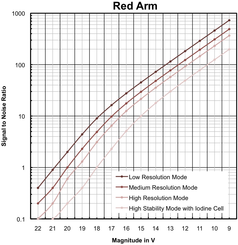
Figure 10. The expected signal to noise ratio (S/N) of SALT HRS as a function of stellar visual magnitude (mv) using the red instrument arm and a variety of operational modes. The calculations are for a wavelength of 725 nm and the low (R~16,000), medium (R~35,000) and high (R~65,000) spectral resolving powers. A blackbody object with surface temperature of 5500K, 2 arcsec FWHM seeing at the fibre input, exposure time of 1800 sec and a telescope airmass of 1.3 are assumed. The sky brightness is calculated assuming the moon to be at first quarter. The S/N is for each extracted half-resolution element at the échelle blaze peak.
Figures 10 and 11 show the anticipated SNR ratio of SALT HRS as a function of stellar visual magnitude (mv). Note the difference in performance of the four instrument modes due to variance in throughput. These values are currently based on predicted instrument efficiencies and are subject to change once on-sky performance is established. Users may simulate HRS observations using the simulator tool available at http://salt4scientist.salt.ac.za/simulators-and-other-tools/.
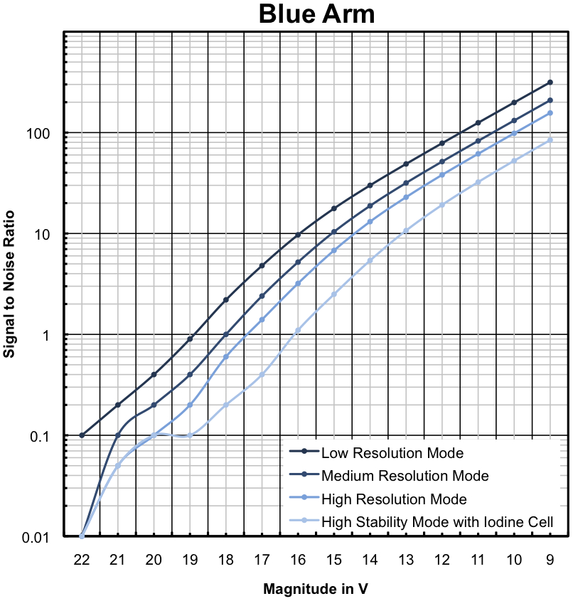
Figure 11. The expected signal to noise ratio (S/N) of SALT HRS as a function of stellar visual magnitude (mv) using the blue instrument arm and a variety of operational modes. The calculations are for a wavelength of 460 nm and the low (R~16,000), medium (R~35,000) and high (R~65,000) spectral resolving powers. A blackbody object with surface temperature of 5500K, 2 arcsec FWHM seeing at the fibre input, exposure time of 1800 sec and a telescope airmass of 1.3 are assumed. The sky brightness is calculated assuming the moon to be at first quarter. The S/N is for each extracted half-resolution element at the échelle blaze peak.
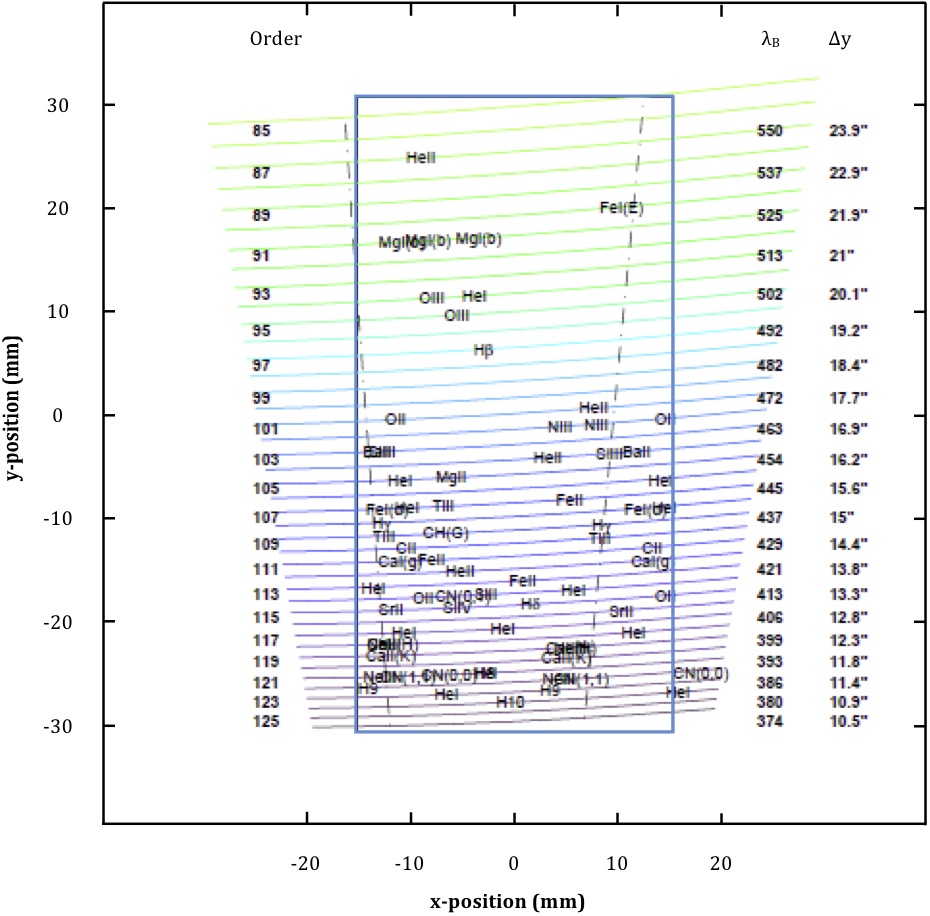
Figures 12 and 13 illustrate the echellogram maps of the red and blue arm spectra as they appear on their 4k x 4k and 4k x 2k detectors respectively. The cross-over wavelength between the two arms is at 555 nm, with the blue arm covering 370-555 nm and the red detector covering 555-890 nm.
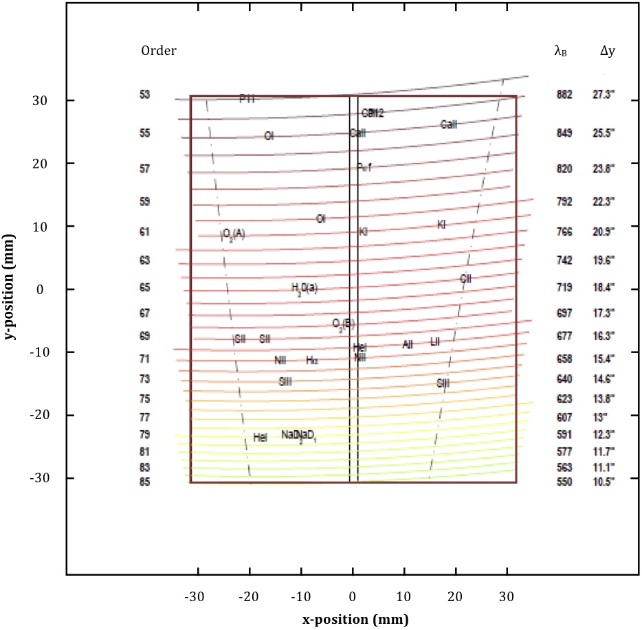
Figure 12. Wavelength coverage for the red arm of SALT HRS. Key spectral features are noted on each image, as are order numbers and the blaze wavelengths λB.
The Berkeley Visible Image Tube camera (BVIT) is a visitor instrument built at the Space Science Laboratory of the University of California-Berkeley. It is a photon-counting camera with a ~1.6-arcmin diameter field of view, capable of very high time resolution (millisec or microsec) photometry with a B, V, R or H-alpha filter. It can be used for objects with magnitudes ranging from V~12-20. BVIT is available for general use. The most accurate and up-to-date information about the instrument, as well as a count-rate estimator, can be found at: http://bvit.ssl.berkeley.edu/.
BVIT does not provide high-precision absolute photometry; however, by observing nearby standard stars, a flux intensity relative precision of ~ 5% can typically be obtained. Every detected photon is assigned a time of arrival and a (x,y) position on the detector, which allows an observer a high degree of post-acquisition data analysis flexibility.
At this time, we are not allowing the BVIT iris size to be altered. The field of view is thus fixed at ~1.6 arcmin in diameter. Note that the two constraints when using BVIT are the global and local count rates. The global rate (sum of all counts on the detector) cannot exceed 2MHz. The local counts from any single source cannot exceed 40kHz. If proposing, please carefully check the field and consider counts from all sources that will be exposed and not solely the target of interest.
The overhead on BVIT data allows for acquisition from one of the larger field-of-view facility instruments (SALTICAM or RSS) as well as an acquisition and count rate check from BVIT.
All SALT Phase-1 proposals must include the overhead times associated with the science observations in the proposed time. The most accurate way to estimate overheads is to use the PIPT tool to build actual Blocks to see how long their execution times are. While Block preparation is not required at Phase 1, the exercise is strongly encouraged to check how feasible the science observations are regarding track times and Block limitations (see Section 2.3) when overheads are included. The main sources of overheads are summarised in Table 13 as well for PIs to get an idea of the involved times. PIs must be especially aware that in addition to pointing and acquisition related overheads, there may be calibration related overheads. The latter may or may not be charged for (see Sections on Calibration Plans, 6.7.2 and 7.8.2), and may or may not affect the available time for science during a track time (e.g. arcs taken after an observation vs. arcs in-between observations).
Please note especially that the basic acquisition time including pointing, focusing, object acquisition, and guidance configuration is 900 sec for MOS and 600 sec in all other instrument modes.
Item | Time (sec) | Comments |
SALTICAM | ||
Acquisition (all modes) | 600 | point, acquire, (guide) |
Dither move | 15 | with ~0.5” accuracy |
Filter change | 11 | |
Readout, Full Frame, Slow | 9.0, 21, 53 | 6x6, 2x2, 1x1 |
Readout, Full Frame, Fast | 8, 14, 26 | 6x6, 2x2, 1x1 |
Readout: Frame Transfer | 0 | minimum exp.times apply |
Readout: Slot Mode | 0 | minimum exp.times apply |
RSS | ||
Imaging acquisition | 600 | point, acquire, guide, RSS config |
Long-slit acquisition | 600 | point, acquire, guide, RSS config |
FP acquisition | 600 | point, acquire, guide, RSS config |
MOS acquisition | 900 | point, acquire, guide, RSS config |
MOS realignment | 360 | re-acquisition, RSS config |
Full RSS config change | 240 | |
Grating angle change | 15 | |
Filter change | 45 | |
Slitmask change | 60 | |
Articulation movement | 71, 38, 142 | 100○ → 0○, 50○ → 0○, 100○ ⇄ 0○ |
Nod along slit, blind offset | 60 | with ~0.5” accuracy |
Arc | 120 | Cal.sys insert + 1 x 60s frame |
Spectral flat | 120 | 5 frames, Cal.sys already inserted |
Readout Full Frame, Slow | 7.3, 17.7, 27, 51 | 4x4, 2x2, 1x2, 1x1 |
Readout Full Frame, Fast | 6.0, 11, 14, 25 | 4x4, 2x2, 1x2, 1x1 |
Readout: Frame Transfer | 0 | minimum exp.times apply |
Readout: Slot Mode | 0 | minimum exp.times apply |
Table 13: SALTICAM and RSS overhead estimates.
An individual observing program will consist of a number of observations of different targets and will be assigned a set of priorities and Moon brightness by the relevant TAC(s). Each partner TAC will have the same breakdown in terms of the percentages of different priorities, and all observations are charged in the same manner. The priorities just influence the likelihood of a given target being observed on a particular night or over several nights. For the upcoming semester, the available science time will be allocated to the different priorities such that 30% for P1 time, 40% for P2 time, and 30% for P3 time with a 1.5 over-subcription rate for P3.
Highest rated Targets of Opportunity (ToO) programs or time critical observations. Once scheduled, and weather permitting, Priority 0 observations will have the highest chance of being observed at the time requested. Examples of such observations might include supernovae, GRBs, and rare periodic phenomena.
Any proposal can consist of time critical observations, but only ones allocated a P0 priority will in general be observed in preference to other priority classes.
Highest rated proposals, which, if scheduled, will have a high chance of being observed in a given night. Such targets will be the most scientifically compelling of all standard priority targets and completion of all P1 programs in a given semester is expected. We hope to achieve 100% completion of P1 proposals.
P2 programs are not as highly rated as P1 by the TACs, but are still considered to be compelling and will have a good chance (>90%) of being completed in a given semester.
P3 programs are lowest priority science as assigned by the TACs, but still worthy of consideration. P3 proposals are deliberately over-subscribed by a factor of 2 in order to always have a full queue, and so will have a 50% chance of being observed in a given semester. Because of the nature of such dynamic scheduling, the easiest P3 proposals are the ones that are likely to be observed in a given night. At best, it is expected that only 50% of P3 programs will be observed.
This is a priority class consisting of “filler” targets, to be done in marginal observing conditions (i.e. poor transparency or bad seeing), not strictly 10-m class science, but deemed to be useful in such degraded conditions. P4 programs will not be charged.
PIs should justify in the application (technical section) why their proposed programs should be considered P4 time (e.g. brightness, observing mode, allowable conditions). TACs will accept or reject the P4 proposals as they see fit. Accepted P4 programs are not guaranteed to be completed in a given semester and observations of P4 programs will only ever be attempted if, at the duty SA’s discretion, there are no other viable P0 - P3 programs that can be attempted.
SALT proposals can only be submitted by astronomers who are members of a SALT consortium institution, or are collaborating with such astronomers. Time can be requested from different SALT partner TACs according to the nature of the collaboration and it is entirely up to the PI and Co-Is to decide what fractions are requested from each TAC. It should be noted, however, that some TACs may look with disfavour on proposals from other partner institutions which request the majority of time from them if the respective Co-Is are minor players in the collaboration.
Programs that are foreseen to extend over multiple semesters will need to be re-applied for and details on the progress of such programs must be provided in the proposal.
At the present time observing time is charged on the basis of completion of requested observing blocks as they appear in the PIPT and SALT Web Manager. It is anticipated that a more realistic time-keeping of actual observing time used will be implemented in the near future, but this is currently awaiting the implementation of the required software.
Details of the requirements for Phase 1 proposals are outlined in a separate document. Once TACs have approved proposals and allocated time according to priority class and Moon brightness, the Phase 2 proposals have to be completed adhering to these allocations. In addition, targets (mandatory or optional) cannot be changed between Phase 1 and Phase 2 unless agreed to by the relevant TACs.
For a Phase 2 proposal, the PIPT will ensure that:
When an imported proposal exists on the user’s computer already, the version on the computer will be replaced with the imported one. Naturally, the user shall be warned beforehand.
Submission of Phase 2 proposals should be done at the earliest opportunity following confirmation of proposal acceptance by the TAC, and must be done by the stipulated deadline. This is crucial for planning of semester observations. ToO programs that do not yet have targets available should submit dummy block(s) so their configurations can be reviewed. For normal proposals, all targets must be submitted at the deadline, but updates may be supplied throughout the semester if required.
All accepted SALT proposals will be assigned a Liaison SALT Astronomer (LSA) who will be the main point of contact between the PI and SALT Ast Ops. Communications regarding the completion of the Phase 2 proposal, the status of the proposal and and issues regarding the observations and data should be communicated with the LSA in the first instance (please refer to Section 11.7).
All communications with SALT Ast Ops should be via email (or telephonically in urgent cases, like ToO alerts) primarily to the SALT Help email address (sa@salt.ac.za). In all cases relating to existing proposals it is imperative that the assigned proposal code is included in the subject of the email. This will ensure that all Ast Ops staff are aware of a request or query even if the particular Liaison SA is unavailable.
For activation of ToO programs, PIs should communicate their request to salthelp@salt.ac.za. For short notice or urgent real-time alerts, the SALT control room telephone number (+27 23 5711356) can be used to contact the duty SA directly.
The PI has two options for data distributions: Normal and Fast. All data will be made available at ftp://saltdata.salt.ac.za/ and are accessible by the contact-PI logging onto that site with their Web Manager username and password.
For “Normal” data distribution, the PI will receive an email when the data has passed through the pipeline in Cape Town. This will typically be within 24 hours of the observations, but may be up to one week later. The PI will receive the raw data, processed data, and documentation including the night log. Information about the current status of the processed data can be found at:
https://wiki.salt.ac.za/index.php/SALT Data Quality
The data will only be guaranteed to be on the ftp site for two weeks. All data should have been downloaded by that time, but if necessary, the PC can have their data posted to their ftp site via their proposal page on the webmanager.
For “Fast” data distribution, the raw data will be made immediately available along with any quicklook product. Once the first observation has been taken for the proposal during a night, the contact-PI will be notified that observations are being made for their proposal. Due to limits on bandwidth and data processing, we ask that only proposals that would truly benefit from this high response time select this option.
The proprietary period of the data will be decided by each individual partner. At this time, none of the partners have yet specified a proprietary period. The PI may specify any proprietary period for their data - we suggest an 18 month proprietary period.
Please notify sa@salt.ac.za of any publication made using SALT data including reviewed papers and conference proceedings.
All science papers that include SALT data which are submitted for publication in refereed science journals must include the following words of acknowledgment:
“All/some [choose which is appropriate] of the observations reported in this paper were obtained with the Southern African Large Telescope (SALT).”
In addition, a footnote symbol should appear after the paper title*, and the following text should be written as a footnote:
*based on observations made with the Southern African Large Telescope (SALT)
If possible, please include the Proposal Code and Principle Investigator for the observations in the paper.
If you use data reduced by the SALT science pipeline or use the PySALT software, please provide a link to http://pysalt.salt.ac.za/ and cite the following paper:
Crawford, S.M., Still, M., Schellart, P., Balona, L., Buckley, D.A.H., Gulbis, A.A.S., Kniazev, A., Kotze, M., Loaring, N., Nordsieck, K.H., Pickering, T.E., Potter, S., Romero Colmenero, E., Vaisanen, P., Wiliams, T., Zietsman, E., 2010. PySALT: the SALT Science Pipeline. SPIE Astronomical Instrumentation, 7737-82
In addition, the following papers provide a description of the telescope and instruments:
SALT:
Buckley, D.A.H., Swart, G.P., & Meiring, J.G. 2006, SPIE, 6267, 32
RSS:
Burgh, E. B., Nordsieck, K. H., Kobulnicky, H. A., et al. 2003, SPIE, 4841, 1463
Kobulnicky, H. A., Nordsieck, K. H., Burgh, E. B., et al. 2003, SPIE, 4841, 1634
RSS FP:
Rangwala, N., Williams, T. B., Pietraszewski, C., & Joseph, C.L. 2008, AJ, 135, 1825
SALTICAM:
O'Donoghue, D. et al. 2006, MNRAS, 372, 151
SALT-HRS:
Barnes et al 2008, Proc of SPIE 7014, 70140K
Bramall et al 2010, Proc of SPIE 7735, 77354F
Bramall et al 2012, Proc of SPIE 8446, doi:10.1117/12.925935
BVIT:
Welsh, B., D. Anderson, J. McPhate, J. Vallerga, O. Siegmund, D. Buckley, A. Gulbis, M. Kotze, and S. Potter, High Time-Resolution Astronomy on the 10-m SALT, New Horizons in Time-Domain Astronomy, Proceedings of the International Astronomical Union, IAU Symposium, Volume 285, p. 99-102, 2012.
McPhate, J., O. Siegmund, B. Welsh, J. Vallerga, D. Buckley, A.A.S. Gulbis, J. Brink, and D. Rogers, BVIT: A visible imaging, photon counting instrument on the Southern African Large Telescope for high time resolution astronomy, Proceedings of the 2nd International conference of Technology and Instrumentation in Particle Physics, hicago, 9-14 June 2011.
Image Quality | See the SALTICAM optical design, Figure A1. 0.3 arcsec (EE50), combined with SALT 0.6 arcsec (EE50), to give 0.67 arcsec image quality, independent of seeing. EE80 shall be no more than 0.5 arcsec. Distortion shall be less than 1 per cent. The mean plate scale shall be 107 micron/arcsec or 9.35 arcsec/mm within 1 per cent. |
Science Field of View | 8 arcmin in diameter |
Guide Star Field of View | 10 arcmin in diameter |
Wavelength range | 320 – 950 nm |
Filters | 8 position filter unit. Available filters include U, B, V, R, I, clear; Sloan u', g', r', i', and z'; Strömgren u, v, b, y, H-beta wide, H-beta narrow, and red extensions SRE1, SRE2, SRE3, and SRE 4; H-alpha; neutral density; and short wavelength interference filters at 340 nm (FWHM 35 nm) and 380 nm (FWHM 40 nm). (see http://www.salt.ac.za/telescope/instrumentation/salticam/specifications/ for filter curves) |
CCD chips | E2V Technologies 44-82 |
Format | 2048 x 4102 x 15 micron square pixels per chip |
Imaging area per chip | 30.7 x 61.5 mm2 imaging area per chip |
Readout capabilities | 2 readout amplifiers per chip |
Mosaicing | 2 x 1 mini-mosaic |
CTE | better than 99.99% |
Full well | 164 and 172 k e-/pix (for CCDs SALT-01 and SALT-02 respectively) |
Dark current | less than 1e-/pix/hr at 160 K |
Readout noise | less than 3.0 e-/pix at 100 kHz (10.0 usec/pix) (slow readout) |
CCD Controller | SDSU II (Leach) from Astronomical Research Camera Inc. |
Sensitivity | Thinned, back-illuminated. Deep depletion silicon. Astro Broad Band anti-reflection coating. |
The lens system reduces the SALT f/4.2 prime focal ratio to f/2, thereby enabling the full 8-arcmin diameter science field of view, as well as almost all of the guide star field of view, to be captured on the 2x1 CCD mosaic. The lenses are made from UV-transmitting crystals, and the CCDs have excellent UV performance, so the instrument is expected to be very efficient at short wavelengths. The optical design is illustrated in Figure A1.
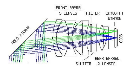
Figure A1. SALTICAM optical path.
Figure A2 shows the fields of view superimposed on the detector and includes:
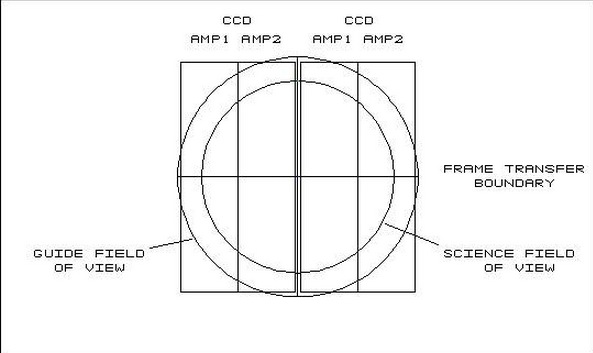
Figure A2. SALTICAM full layout.
The detector is a 2x2 mosaic of 2kx4kx15 micron pixel CCD 44-82 chips from E2V Technologies. These devices are thinned, back-illuminated and coated with the E2V Astro Broad Band coating. They are also deep-depletion devices for better near-infrared sensitivity and lower fringing. A schematic of one of the chips is shown in Figure A3.
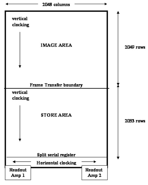
Figure A3. SALTICAM schematic for one of the two CCDs.
For moderate time resolution on the order of a few sec, frame transfer (FT) operation is used. This is explained by the left hand diagram in Figure A4: a mask (shown in grey) covers the lower half of each chip. At the end of each exposure, the image in the top half of the chip is rapidly (200 millisec) shifted to the lower half where it is readout while the next image in the top half accumulates during the next exposure.
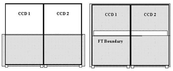
Figure A4. SALTICAM schematic for frame transfer (left) and slot mode (right). The gray regions are masked.
Even faster sampling can be obtained with so-called slot mode: in this mode a mask is advanced over the entire chips except for a slot just above the frame transfer boundary. Instead of half frame transfers at the end of each exposure, 144 rows are moved and this allows exposure times as short as 100 millisec. The slot position is illustrated in the right hand diagram in Figure A4. Figure A5 shows a schematic of the slot mode readout:
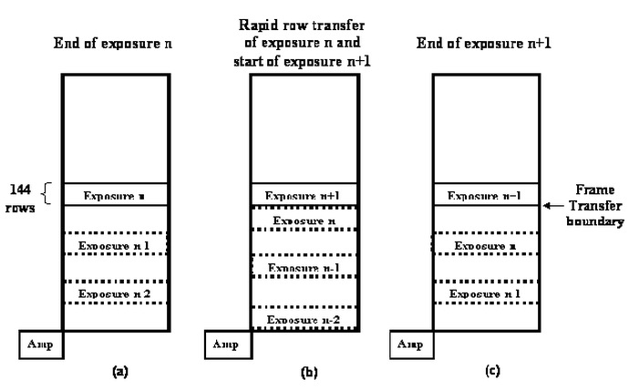
Figure A5. SALTICAM schematic for slot mode readout.
Figure A5, panel (a) shows the situation at the end of exposure n in one of the 4 amplifiers of the SALTICAM CCDs. The 144 rows indicated are transferred in about 15 millisec over the frame transfer boundary which is supposed to be aligned with the lower edge of the slot. At the end of this operation (panel (b)), exposure n lies in the 144 rows below the FT boundary, and exposure n+1 begins. During exposure n+1, the 144 rows next to the readout register (indicated by exposure n-2 but in reality n-6) are read out, and the other data sections slowly scroll down by 144 rows. At the end of exposure n+1, the situation is then as in panel (c) which is the same layout as in panel (a) except that n is now replaced by n+1.
Of course both FT mode and slot mode techniques require field of view to be sacrificed for time resolution: in FT mode, half the field of view is lost; in slot mode, only the slot is available for imaging. The intended use of slot mode is to position a rapidly varying target star and a brighter nearby companion star in the slot to perform differential photometry of the variable with respect to the comparison star. The telescope rho stage can be rotated to locate comparison stars at arbitrary position angles within the slot.
"Typical" instrument and system efficiencies are shown in Fig. A1 and were calculated for the on-axis field position using:
Fig. A6 shows SALTICAM efficiency as the product of the optics and the CCD curves. For reference, RSS performance taken from Fig. 5 of the PFIS PDR Instrument Description Document is also shown.
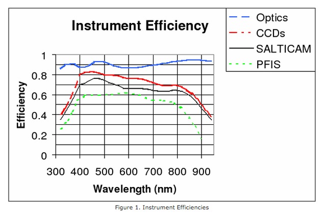
Figure A6. SALTICAM instrument efficiency with PFIS (now RSS) for comparison.
Below, Fig. A7 shows overall efficiency based on:
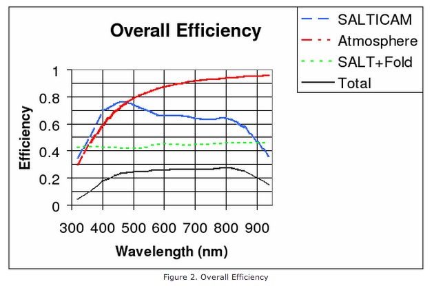
Figure A7. SALTICAM overall efficiency (including telescope optics and atmosphere).
The moving pupil inherent to the basic operation of SALT presents special problems for doing photometry with SALTICAM. While it is true that if the tracker position is known at all times, the fraction of the primary mirror within the pupil can be calculated (including gaps between mirrors) and the photometric "response" function of the telescope can be worked out. However, this assumes equal reflectivity for all mirrors; clearly this will not be true and furthermore it will be variable as the cycle of mirror recoating runs. (Typically, at least one and possibly two segments per week will be recoated).
Measuring reflectivities of mirrors is an uncertain process so it seems very difficult to provide calibrations sufficient to estimate the response function to at least 1 per cent (preferably better) for all tracker positions.
So those carrying out photometry with SALTICAM should bear in mind:
SALT Proposal Info: 2013 Semester 2