Southern African Large Telescope
Title: | Proposal Information for SALT Call for Proposals: 2026 Semester 2 Phase 1 Deadline: 7 August 2026, 16:00 UT Phase 2 Deadline: 16 October 2026, 16:00 UT |
Author(s): | SALT Ast Ops |
Doc Number: | 2430AB0001 |
Version: | 1.0 |
Date: | 25 June 2026 |
Approved: | Danièl Groenewald (Head of SALT Astronomy Operations) |
Abstract
This document provides information to potential SALT proposers that will assist in making their Phase 1 & 2 proposals for 2026 Semester 2 (1 November 2026 – 30 April 2027). It summarises the essential features for new users, the latest instrument status, and changes from previous semesters. It incorporates the latest experiences from SALT Astronomy Operations regarding telescope and instrument performance. The document also includes proposal policies and related information. The SALT website should be consulted from time to time for further updates. The Phase 1 proposal deadline is 7 August 2026 at 16:00 UT. The Phase 2 proposal deadline is 16 October 2026 at 16:00 UT.
Table of Contents
How is SALT different from most other large telescopes?
What is SALT especially suited for?
How to get time and observations?
Strategic tips, tricks and hints
Historical target distribution on the sky
Historical Priority completeness fractions
1.3 Current status of the telescope
1.3.2 Instrument and mode availabilities
1.3.3 Other current information
1.5 Schedule for 2026-1 semester
1.6 Software download and valuable links
Proposal tools and information:
2. Essential Concepts Regarding SALT
2.1 SALT as a fixed altitude telescope
2.2. SALT as a service telescope
2.4 Open and closed loop tracking
2.5 Visibility and track length
3. SALT Proposal Guide: Definitions and Procedures
3.2 Phase 1 late submission policy
3.3.2 Large Science Programs (LSP)
3.3.3 Director’s Discretionary Time (DDT) proposals
3.3.4 Commissioning (COM) proposals
3.3.5 Science Verification (SV) proposals
3.5 Concept of “Optional Targets”
3.6.1 Definitions of Lunar illumination
3.6.2 Seeing conditions at Sutherland
3.6.3. Definition of cloud cover conditions
3.7 Phase 1 proposal preparation and submission
3.8 The procedure between the two proposal phases
3.9 Phase 2 proposal preparation and submission
3.10 Data distribution and reduction
3.10.1 Data proprietary period
3.10.2 SALT pipeline data reduction
3.10.3 SALT data reduction user packages
3.11 Publication and acknowledgment policy
Science paper acknowledgements
4. Telescope Performance and Observing Constraints
6.2 Characteristics and performance
6.3 Readout speed and gain settings
6.4 Available instrument modes
6.6 Photometric accuracy and flat-fielding
6.10.1 Features of SALTICAM calibrations
6.10.2 Current SALTICAM calibrations plan
7. RSS: Detector replacement is happening in 2026-1
7.3 Characteristics and performance
7.7 Available instrument modes
7.7.1 Narrow-band or clear imaging
7.7.2 Long-slit spectroscopy (LS)
7.7.3 Slitmask IFU spectroscopy
7.7.4 Multi-object spectroscopy (MOS)
7.7.5 Polarimetry imaging / spectropolarimetry
7.7.6 High-speed imaging and spectroscopy
7.10 Blind offsets, dithering and nodding
7.11.1 Features of RSS calibrations
7.11.2 Current RSS calibration plan
8.2 Characteristics and performance
8.4.1 Caveats and recommended readout modes
8.5.1 Low resolution mode (LR)
8.5.2 Medium resolution mode (MR)
8.5.3. High resolution mode (HR)
8.5.4 High stability mode (HS)
8.5.5 HRS Resolution Measurements
8.7 Stability of radial velocities (RVs)
8.9.1 Features of HRS calibrations
8.9.2 Current HRS calibrations plan
A.1 Glossary and abbreviations
A.3 SALT Telescope and the Array Management System (SAMS)
A.4 SALT Tracker and Instrument Payload
A.5 SALTICAM Technical Information
High time-resolution modes: Frame Transfer and Slot mode
A.8 Narrow-band filter transmission curves
Quick Start
1.1 How to read this document
This document is organised as follows. Sections 1 – 3 form the introduction to SALT (Southern African Large Telescope) and describe the proposal process. Sections 4 – 10 cover the details on the telescope and instrument characteristics. The appendix gives a glossary, a list of the SALT partners, and technical details of the instruments.
For recurrent users, the most interesting sections will be the status of the current semester, including a list of changes from the last call, presented in Sec. 1.3. In addition, each instrument section gives the specific current status for that instrument at the beginning of the relevant section (6.1 to 8.1). At the end of each instrument section the current calibration plan is given. Important dates and deadlines can be found in Sec. 1.5. The PIPT has been updated since last semester, PIs are welcome to use our latest version (see Sec. 1.6). It is also advisable to re-familiarise yourself with the details on the proposal submission (Sec. 3) and to take note of the important information given in bold font.
If you are a recurrent user but have not applied for time lately, you can refresh your memory by browsing the tips presented in Sec. 1.2 and the relevant telescope and instrument performance sections for any news.
New or first-time users should make themselves familiar with the specifics of SALT as a telescope (See Sec. 2 on how SALT differs from other telescopes of its class and what its limitations are, and Sec. 4 on SALT’s characteristics and performance) and the details of how to write the proposal (Sec. 3). Section 1.2 gives useful tips on how to make best use of the telescope and its instruments and how to increase the likelihood to get time allocated and the observations executed. Both the section on how calibrations are done or requested (Sec. 5) and how to calculate overheads (Sec. 9) are important for calculating the overall time request. Every instrument section presents first an overview of the status of that instrument (what is available in this semester, what to look out for and possible caveats), followed by detailed descriptions on available modes, filters (including descriptions on performance), etc. The last subsections containing the information on what kind of calibration observations for each instrument are offered for free and which calibrations the user can choose for themselves are also very important. A glossary on SALT-specific expressions and acronyms can be found in the Appendix as well as technical details about the instruments.
1.2 Overview and tips
SALT is an optical 10-m class segmented-mirror telescope situated at a dark site in Sutherland, South Africa. SALT is especially suited for spectroscopic and high time-resolution observations. SALT is fully queue-scheduled with possibilities for real-time input from the PIs and fast turnaround data delivery. Target visibility is in the range of DEC = +11 to –76 deg.
How is SALT different from most other large telescopes?
- How long a given target is available during a given night and how long its continuous visibility (track) is, are both dependent on the target’s declination. The availability during the night ranges from 4 hours for Equatorial and DEC < –65º targets to typically 1–1.5 hours in a rising or setting track elsewhere. On the other hand, the continuous visibility (track) of a target is 2–3 hours in between –60º < DEC < –76º, while for Equatorial objects a maximum time on-source per single visit is about 45 minutes. Be sure to read the essential concepts in Sec. 2.5. It is especially important to grasp the meaning and difference of visibilities and tracks.
- The SALT pupil changes during an observation (Sec. 2.3). Relative calibration is possible by e.g. using comparison stars in imaging, and spectral shapes can easily and reliably be calibrated using spectrophotometric standards. Accurate absolute (spectro-)photometric calibration should be done using supplementary information about the target fields from elsewhere.
- The primary mirror is segmented. An active mirror alignment system (SAMS) was implemented in April 2016 and the PSF is very stable during the night. Nevertheless, Sutherland remains a site with modest seeing (median value at Zenith about 1.5 arcsec). PIs should recognise that while both imaging and faint object spectroscopy with SALT are more viable now than in the past, the size of a typical PSF still means the signal-to-noise (S/N) of faint point-sources is lower compared to observations done in sub-arcsec seeing.
What is SALT especially suited for?
- The large collecting power and dark skies (V = 22.0 mag/sq.arcsec at zenith during dark time and Solar minimum) mean that diffuse low surface brightness objects are ideal for very competitive results.
- Likewise, brighter objects where most of the light is above background regardless of the PSF size and shape, can be observed very efficiently.
- There are several modes of spectroscopy, including high-speed, high-resolution, multi-object, Fabry-Pérot (currently unavailable) and polarimetric capabilities. Some of these observing modes are rare on large telescopes. Most modes are available all of the time; SALT is capable of changing modes and instruments on-the-fly in less than a minute, as well as combining certain modes.
- Read Sections 4.3, 6.7, 7.8 and 8.8 for information on instrument sensitivities and, above all, familiarise yourself with the Instrument Simulators available at http://astronomers.salt.ac.za/software/.
How to get time and observations?
- SALT is owned by a consortium. All SALT time is allocated by a SALT Partner, or multiple partners. SALT proposals can only be submitted by astronomers who are members of a SALT Partner institution, or are collaborating with such astronomers. See Sec. 3 for the application process with deadlines twice per year. The PIPT software must be used for submissions.
- There is a modest amount of open and free Director’s Discretionary Time (see Sec. 3.3.3) available outside of the normal proposal process. Note that investigators for DDT proposals need not belong to a SALT Partner.
- There is also uncharged filler time (P4, Sec. 3.4) available for accepted proposals.
- SALT is 100% queue-scheduled. You apply for a given amount of time, not for certain dates, though time windows can be specified for time-restricted targets. You do not come to observe yourself, but will receive the data after each observation has been taken. This also makes long-term monitoring possible.
Strategic tips, tricks and hints
- Over the past semesters, bright time has been undersubscribed. If you have targets that can be observed in fairly bright moon conditions (e.g. >70% Lunar illumination) you have a fairly good chance of getting data.
- Programs that are possible to do in poor seeing (>2.5”) also have lower competition.
- Much of the observational competition is driven by the distribution of targets on the sky. Check the historical figure below. If you have targets in low-target-density regions, you will have higher chances of getting your observations done.
- The PIPT allows you to submit more blocks than your time allocation: you can define a pool of optional targets. This is especially useful if you have a target list with a wide RA-range.
- You should plan for these optional targets during your Phase 1 by, for example, submitting a sample of 50 objects, but telling your TAC that you will get the necessary statistical science from any 15 of them. Having this background pool will greatly increase your chances of getting those 15 done, and it may also be an advantage to show your TAC that you are using your Partner time wisely.
- If you have an approved proposal, the PIPT also allows you to submit P4 time. There is no limit for this time, and it does not come out of the Partner share allocations. The time is “free” if you just convince your TAC to accept the project in principle. See Sec. 3.4. P4 blocks will only be done if there is nothing else available in the queue, due to gaps in the queue, or due to poor conditions. Hence, the most effective P4 programs comprise:
- short blocks, say, 15–30 min long which are easy to plug into gaps
- bright targets, say, 10–17 mag, easily done in any conditions
- a large pool over a wide RA-range to have something available at any time.
Historical target distribution on the sky
Figure 1.1 shows a smoothed “heat-map” of the number of proposed Observing Block (Sec. 2.6) visits over Semester 2023-2. The distribution is very non-uniform. Areas with a very high number of proposed visits include the Magellanic Clouds, the Galactic Bulge, some Deep Fields and Equatorial fields. It is thus not possible to execute all of the blocks even if they had the highest priorities. Note however that track times (see Sec. 2.5) are much longer at deep southern declinations, while visibilities are longer at the equator, increasing the likelihood that such targets get observed over those in oversubscribed areas.
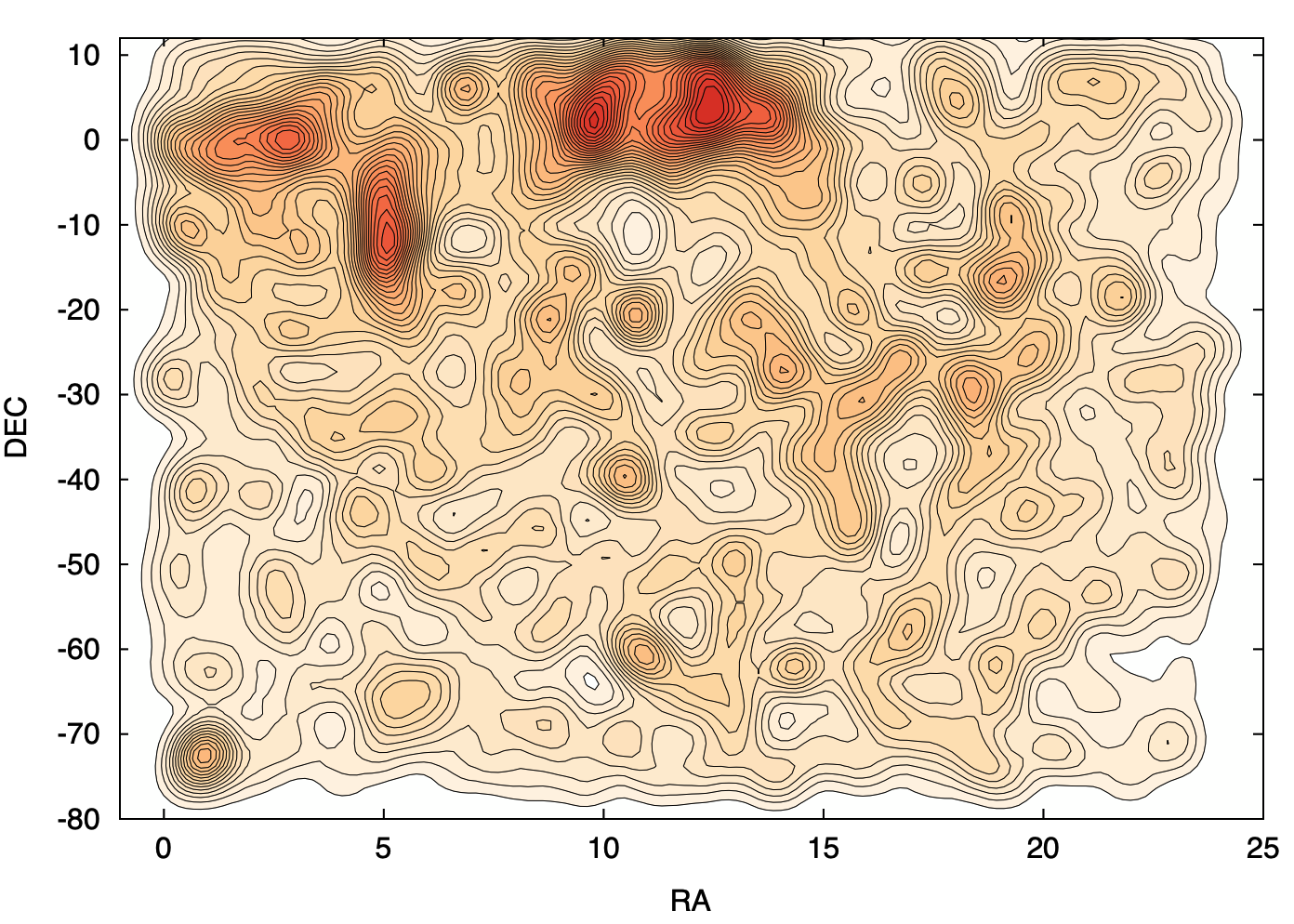
Figure 1.1: Smoothed target distribution for the 2023-2 semester.
Historical Priority completeness fractions
Time allocation is done by Priorities (Sec. 3.4). Figure 1.2 shows the average realised completeness of time per priority over five past semesters. For P0 (time critical observations only) the completeness refers to the triggered observations.
Figure 1.2: Completeness of Observing Blocks by priority, for 2022-2 to 2024-2. The P3 completion is divided by 3, as it’s over-subscribed by a factor of 3.
1.3 Current status of the telescope
1.3.1 Changes from last call
- Update on SALT’s Optical Performance:
Following the 2025 maintenance shutdown, SALT has been found to be facing a serious performance issue due to a deterioration in the coatings of the Spherical Aberration Corrector (SAC) optics. The SAC mirrors have advanced multi-layer coatings, expected to last the lifetime of the telescope, and the SAC was never designed for easy access or long-term servicing beyond dust cleaning. However, after 20 years of exposure, one of the coating layers in one of the mirrors has now failed internally, and another mirror shows early signs of degradation. This is not something that could have been prevented.
This deterioration now significantly impacts sensitivity, particularly for fainter targets.
A strategic restoration project (ReSAC) is being developed to fully recover and enhance SALT’s performance. In the interim, proposers are encouraged to factor in the reduced throughput when planning observations. The SALT instrument simulators have been updated to reflect the current throughput and will continue to be maintained accordingly.
We remain committed to transparency and scientific excellence, and will keep the community informed as the ReSAC initiative progresses.
- The new RSS monolithic detector will be installed.
We plan to integrate the new detector into RSS towards the end of semester 2026-1, with installation currently scheduled for 1 September 2026. It is however unlikely that RSS will be available at the start of semester 2026-2 while the detector is installed, commissioned, and verified for science operations. Further details regarding the installation timeline and expected instrument availability will be communicated to users as they become available. We are excited to be approaching this major upgrade, which will significantly enhance the capabilities of RSS.
- We are pleased to announce that the new SMI-300 IFU will be available for shared-risk observations during the 2026-2 semester.
Interested SALT users who would like to examine one of the commissioning datasets are welcome to contact the SALT Helpdesk and request access to the data. Please note that these datasets remain proprietary and are currently being used for the preparation of the SMI-300 science verification and instrumentation papers. Accordingly, the data may not be published, distributed, or otherwise shared with third parties without the permission of the Science Verification team. Furthermore, results based on these data may not be presented at conferences, included in publications, or otherwise made public prior to the publication of the science verification paper, unless explicit permission has been granted by the Science Verification team.
- The NIRWALS detector is being replaced.
As a result, the instrument will be unavailable for science observations until further notice. Further updates will be provided as they become available.
- SALTICAM modes.
SALTICAM modes Frame transfer and Slot mode are not offered anymore. Users are advised to utilise these modes on RSS, which can also be used in imaging mode.
- Blocks for a Phase 2 proposal can be submitted with the AEONlib Python library.
With the exception of some advanced edge cases you can define blocks as a Python object and easily submit them.
- If you have missed a semester, check the “Changes from last call” in the previous versions of this document archived here.
1.3.2 Instrument and mode availabilities
SALT has an active mirror alignment system with edge sensors which keeps its image quality stable during the night. RSS optics are cleaned every 18–24 months; the most recent service was performed in April 2025 (see Sec. 4.3 for the effects of servicing on the throughput measurements).
SALTICAM, RSS and HRS will be available in the upcoming semester, but with the following restrictions. More details can be found later in the document in relevant sections.
- RSS will be available from the start of 2026-2 using the new detector and control system. The entire 2026-2 semester will be shared risk science time with RSS whilst we iron out any teething issues and confirm the desired data quality.
- A slitmask IFU is available to use with RSS.
Users intending to use this IFU please read section 7.7.3 and document SMI for the SALT Call for Proposal Phase 1. Users may also be interested in the user handbook which contains crucial specification and information on the data reduction process (for SMI-200 only). It can be found here: SMI -200 Handbook
- Polarimetry –– Spectropolarimetry is available for point-source, compact object and extended object spectropolarimetry. We will further prioritise the available polarimetric mode characterizations by the proposals being submitted for 2026-2. We ask that those interested in any other modes contact salthelp@salt.ac.za with their wishes by the same Phase 1 deadline.
- Accuracy of multi-object spectroscopy –– Rotational field drift is corrected by our dual guide probes. The accuracy of MOS acquisition and alignment is ~0.1” and can be routinely done if the PI-supplied reference stars have accurate astrometry. See Sec. 7.7.4 for details.
- No non-sidereal tracking.
- Restricted detector modes for HRS –– We continue to restrict the detector setups to a single combination chosen to provide the best scientific results: Single amplifier, low speed readout, 1x1 binning. PIs requiring other combinations need to clearly justify their request in the technical section of their Phase 1 proposal. See in particular Sec. 8.4. These non-supported mode requests will be reviewed by the SALT Operations team, who will then decide which extra mode(s) they are able to support for the 2026-2 semester. Please note that supporting a non-default mode (i.e. allowing these observations) does not mean that pipeline products will be made available. PIs interested in non-standard modes are encouraged to contact salthelp@salt.ac.za before the Phase 1 deadline to discuss options.
- PIs interested in using any currently unavailable modes are invited to contact salthelp@salt.ac.za to discuss possibilities, after reading the applicable instrument sections below.
1.3.3 Other current information
- 15-20 hours will be set aside specifically for DDT/GWE proposals this semester. Please see Sec. 3.3 for more information.
- Breakdown of priority times: 40% for P0+P1 time, 40% for P2 time, and 20% for P3 time with a factor 3 over-subscription rate for P3.
1.4 Looking into the future
- More polarimetric modes are becoming available – users are encouraged to contact salthelp@salt.ac.za to indicate their priorities.
1.5 Schedule for 2026-2 semester
The SALT semester definitions are:
Semester 1: 1 May to 31 October (deadline late-January)
Semester 2: 1 November to 30 April (deadline late-July)
The current period, 2026 Semester 2 (i.e. for proposal codes starting with 2026-2), runs from:
1 November 2026 to 30 April 2027.
The call for SALT proposals for 2026-2 opens on:
25 June 2026.
The deadline for Phase 1 proposal submissions is:
7 August 2026 at 16:00 UT.
The deadline for Phase 2 proposal submissions is:
16 October 2026 at 16:00 UT.
Late Phase 2 submissions will not be activated and will therefore not be observed, unless discussed with the liaison astronomer before the deadline.
1.6 Software download and valuable links
Proposal tools and information:
- Online FAQ regarding proposal preparation and submission can be found at http://astronomers.salt.ac.za/proposals/faq/
- A guide on how to maximise one’s chances to get SALT time: http://ssc2015.salt.ac.za/wp-content/uploads/sites/77/2015/06/Vaisanen-MaximizingChances.pdf
- Tips and tricks for preparing a proposal: http://astronomers.salt.ac.za/proposals/tips-and-tricks/
- Time allocation criteria: http://astronomers.salt.ac.za/proposals/time-allocation-criteria/
- Web manager: https://wm-new.salt.ac.za. To create an account you can register at https://wm-new.salt.ac.za/register.
- Progress report for long-term proposal: see the proposal’s page in the Web Manager (https://www.salt.ac.za/wm/)
- PIPT: the proposal and observation preparation tool and can be downloaded from https://astronomers.salt.ac.za/software/#PIPT; the online manual is available as html or pdf file. Please use version 6 (or higher) if you plan to use the Slitmask IFU.
- The Java environment provided by Azul:
https://www.azul.com/downloads/?package=jdk#zulu; preferably use version 11
- The template for technical and scientific justification (Phase 1) can be downloaded in various formats and for different proposal types from
http://astronomers.salt.ac.za/proposals/proposal-templates/
- Simulators for SALTICAM, RSS and HRS can be downloaded from http://astronomers.salt.ac.za/software/.
- VPH grating simulator:
http://www.sal.wisc.edu/PFIS/docs/rss-vis/ebb/pfis/observer/specsim.html
- For MOS slit mask preparations use either PySlitMask (https://astronomers.salt.ac.za/software/#PySlitMask) or RSMT (https://astronomers.salt.ac.za/software/#RSMT)
- MOS restricted declination-dependent availability of field orientation: http://astronomers.salt.ac.za/wp-content/uploads/sites/71/2014/08/SALT_PA_Visibility.pdf
- MOS Phase 2 FAQ page: http://astronomers.salt.ac.za/proposals/mos/
- The Visibility Calculator can be downloaded from
https://astronomers.salt.ac.za/software/#VisibilityCalculator
- Finding charts can be made using the Finder Chart Tool, see https://astronomers.salt.ac.za/software/#FinderChartTool. However, in most cases you should be able to generate them from the Acquisition tab in the PIPT.
- Available dither patterns: http://astronomers.salt.ac.za/proposals/dither-patterns/
- Position angle requirements are explained in http://astronomers.salt.ac.za/wp-content/uploads/sites/71/2014/08/SALT_PA_Visibility.pdf
- Sutherland seeing conditions: Catala et al. 2013
- Current information on availability of DDT:
http://astronomers.salt.ac.za/proposals/directors-discretionary-time/
- AEONlib (https://github.com/AEONplus/AEONlib/) can be used to submit blocks with a Python script.
Further reading
(Note that Web manager credentials are needed to access the science wiki pages):
- SALT
- Telescope: Buckley et al 2006
- SAMS: http://www.salt.ac.za/news/sams-project/ and Gajjar et al. 2016
- SALTICAM
- Instrument: O'Donoghue et al 2006
- Flat-fielding: https://sciencewiki.salt.ac.za/index.php/Status_of_Flat_Field_commissioning
- Photometry: https://sciencewiki.salt.ac.za/images_sciencewiki.salt.ac.za/2/2f/Salticam-phot-nov2011.pdf
- RSS
- Instrument: Burgh et al 2003, Kobulnicky et al 2003
- Stability: http://wiki.salt.ac.za/images_wiki.salt.ac.za/3/31/RSS_stability.pdf
- Fringing: https://sciencewiki.salt.ac.za/images_sciencewiki.salt.ac.za/1/12/SALT_RSS_fringing.pdf
- Commissioning report: https://sciencewiki.salt.ac.za/images_sciencewiki.salt.ac.za/1/17/Rss_comm_report_v1.1.pdf
- RSS MOS
- Phase 2 detailed information and FAQ: http://astronomers.salt.ac.za/proposals/mos/
- HRS:
- Instrument: Barnes et al 2008, Bramall et al 2010, Bramall et al 2012, McCracken et al 2017
- Radial velocity stability: http://www.saao.ac.za/~akniazev/pub/HRS_MIDAS/HRS_stability.pdf
Data reduction:
- All data will be available at ftp://saltdata.salt.ac.za/ (PC login required)
- The new version of the RSS science data pipeline is working now and users receive 2D wavelength calibrated data. The current RSS science data pipeline is a Pythonised version of the RSS long-slit reduction pipeline package from Kniazev 2022. Users can find more information on the science pipeline on https://astronomers.salt.ac.za/software/rss-pipeline/.
- Information on PySALT, the former primary data reduction package, and its usage can be found on https://astronomers.salt.ac.za/software/pysalt-documentation/ and https://sciencewiki.salt.ac.za/index.php/PySALT_Data_Tutorials
- Data reduction FAQ: http://astronomers.salt.ac.za/data/data-reduction-faq/
- Analysis software for spectro-polarimetry: https://github.com/saltastro/polsalt
- Line atlas for RSS: http://pysalt.salt.ac.za/lineatlas/lineatlas.html
- HRS:
- Pipeline description: http://astronomers.salt.ac.za/software/hrs-pipeline/
- MIDAS HRS data reduction: Kniazev et al. 2016a, 2016b
- PyHRS description: Crawford et al. 2016 (no longer supported)
Miscellaneous:
- Live status of the telescope: http://astronomers.salt.ac.za/status/
1.7 Communication details
General:
- Head of Astronomy Operations (or Manager): saltastrohead@salt.ac.za (Danièl Groenewald)
- SALT Astronomers working at the observatory / SALT Operations: sa@salt.ac.za
- Helpdesk queries: salthelp@salt.ac.za
Specific communications:
- Large Science Programs should be announced to the Head of Astro Ops at saltastrohead@salt.ac.za (Danièl Groenewald) at least 2 weeks prior to the Phase 1 deadline (see Sec. 3.2.3)
- DDT issues and submission: ddt@salt.ac.za
- ToO alerts: send email to the SALT Help email address (salthelp@salt.ac.za or sa@salt.ac.za which end up in the same place). This will ensure that all Astronomy Operations staff are aware of a request or query even if the particular Liaison SA is unavailable.
- Proposal issues:
- General: salthelp@salt.ac.za or sa@salt.ac.za (which end up in the same place). In all cases relating to existing proposals it is imperative that the assigned proposal code is included in the subject of the email.
- During Phase 1 submission stage: salthelp@salt.ac.za (Previous submissions will have been assigned a program code – in that case, that code must be provided in the subject line).
- During Phase 2 submission stage: email in the first instance your Liaison SALT Astronomer using sa@salt.ac.za or salthelp@salt.ac.za, adding the proposal code to the subject of the email.
- During observations: All communications with SALT Astronomy Operations should be via email primarily to the SALT Help email address (salthelp@salt.ac.za or sa@salt.ac.za which end up in the same place). In all cases it is imperative that the assigned proposal code is included in the subject of the email. This will ensure that all Astronomy Operations staff are aware of a request or query even if the particular Liaison SA is unavailable.
Publications:
- Please notify salthelp@salt.ac.za of any publication made using SALT data including reviewed papers and conference proceedings.
2. Essential Concepts Regarding SALT
2.1 SALT as a fixed altitude telescope
SALT is a fixed altitude telescope and is closely modelled on the Hobby-Eberly Telescope (HET) concept. The design comprises a spherical primary mirror mosaic of 91 identical 1 m wide hexagons, tilted at a constant zenith distance (37 degrees), with azimuthal rotation only for target acquisition, see Fig. 2.1. The target is then tracked by moving the instrument payload at the primary focus (“tracker”, see Fig. 2.2). The payload tracker has a range of +/- 6 degrees. The spherical aberration corrector (SAC) provides an F/4.2 beam with an 8 arcminute field of view at prime focus.
SALT can access ~70% of the sky observable at Sutherland, but only during specific "windows of opportunity" (see Sec. 2.5). Objects are not always accessible by SALT, even though they may be above the horizon. However, the dates an object can be observed during the course of a year are almost identical to that of a more traditional telescope.
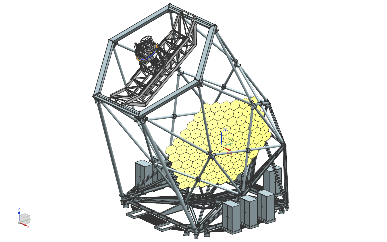
Figure 2.1: SALT telescope structure with instrument payload and tracker. The telescope can move only in azimuth while the tracker can only move up and down the structure which supports it.
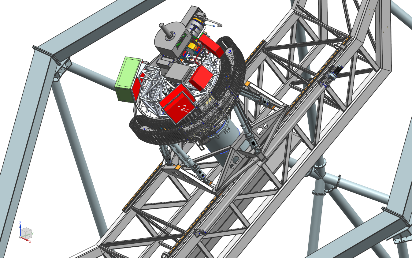
Figure 2.2: Tracker with instruments (payload); the RSS is visible at the top and the SAC is the grey cylinder underneath.
2.2. SALT as a service telescope
SALT is operated as a queue-scheduled telescope. There is a dedicated group of 8 SALT Astronomers that observe the targets for each individual program, depending on the current weather conditions and the constraints placed by the PI, on any given night. Each target is assigned a priority, a score that is based on the particular requirements of the proposal, the time that the target is available for the rest of the semester, and other factors. Thus, at any given time during the night there will be a list of targets to choose from, and the SALT Astronomer working at the telescope is responsible for observing the highest scoring and highest priority target that matches the observing conditions to collect the data on behalf of the PI. This queue-scheduled operation of SALT makes use of all available observing time in the most efficient manner.
2.3 Moving pupil
As part of the SALT design, the pupil (that is, the view of the mirror as the tracker sees it) moves during the track and exposures, thereby constantly changing the effective area of the telescope (see Fig. 2.3). Because of this, accurate absolute photometry and spectrophotometry are not feasible. Photometric calibration of imaging must be done using external data of the same field, though internal colour information can be obtained using filter cycles in the case of short exposures (see https://sciencewiki.salt.ac.za/index.php/File:Salticam-phot-nov2011.pdf for more details). Spectrophotometric standards are routinely taken and can be used for relative spectral (shape) calibration, but not for absolute flux calibration.
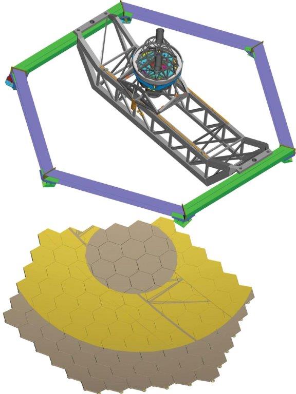

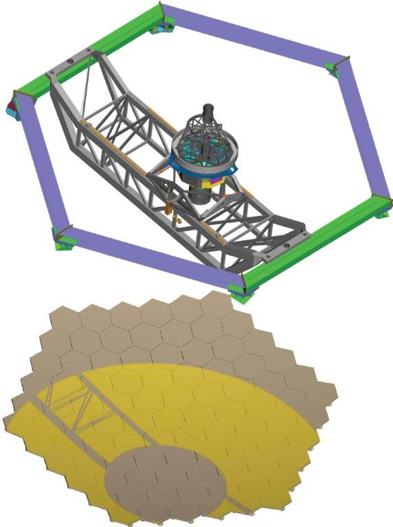
Figure 2.3: The pupil (yellow) for three different tracker positions. The grey areas are non-illuminated parts of the mirror.
2.4 Open and closed loop tracking
SALT tracks in two modes: closed loop and open loop. In closed loop, the telescope position is controlled automatically by a guidance probe and focus can be adjusted as required. This is the standard mode for spectroscopy. In some cases when doing imaging, guidance may not be available and then open loop tracking is employed. In this case the position and focus may drift slightly and short exposure times are recommended (see, e.g., Sec. 6.9).
2.5 Visibility and track length
The altitude restrictions on SALT (47º to 59º) place observing constraints in terms of instantaneous sky access in Hour Angle and Declination, which is shown in the visibility annulus or so-called SALT “toilet seat” diagram in Fig. 2.4. Prominent astronomical objects are marked at their respective declinations. Only objects inside the annular region are observable by SALT at any given time. Objects at southerly declinations are visible for longer periods (several hours, e.g., the LMC) compared to those at northerly declinations, where the average time for a single track is only 50 minutes. For all except the most northerly or southerly declinations, objects can potentially be observed twice a night at favourable times of the year. The airmass over SALT’s elevation range varies from 1.17 to 1.37 with a mean of ~1.25.
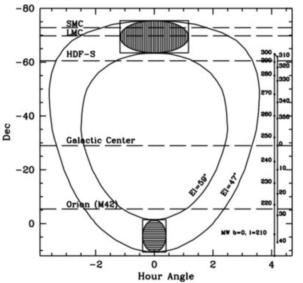
Figure 2.4: The visibility annulus of objects observable with SALT, as a function of declination and hour angle. The hashed regions show the range of motion for the tracker at two different declinations.
The total maximum observing time, or visibility, for a celestial target is defined as the time it takes to transit the annulus, which is dependent on the Declination. While the telescope can access any point within this visibility annulus, the length of time a target can be tracked is not only restricted by the boundaries of this annulus, but also by the tracker movement (see Fig. 2.4) since the telescope structure cannot be moved while observing. Thus the maximum track length for an object, is equal to or shorter than the visibility time. The two hashed regions in Fig. 2.4 are examples of areas that can be reached by moving the tracker alone (that is, without moving the telescope). In other words, it is this maximum track time (and not the visibility) that defines the maximum length of an observing block (see Sec. 2.6). Of course, while the target is still visible, a new pointing can lengthen the total observing time by moving the telescope structure to a new azimuth position and starting a new observation.
For example, Equatorial targets lie in the zone where two visits per night are possible (e.g., the Galactic Centre target in Fig. 2.4), but they have highly constrained track times with, in practice, around 45 mins maximum to use for an exposure (in addition to the pointing/acquisition), see Fig 2.5. The longest track times of more than 2.5 hours can be achieved for very southern targets.
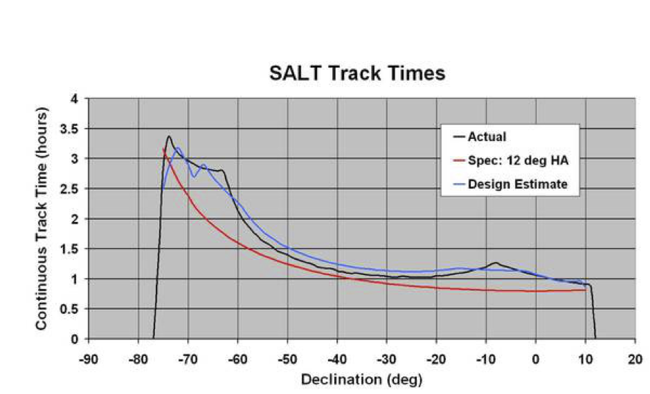
Figure 2.5: The “actual” total maximum track time for objects as a function of Declination.
For planning purposes it is essential that the PIs use the Visibility Calculator (see Sec 3.7), which gives more accurate information than Fig. 2.5. Figure 2.6 shows a snapshot with the target information to the left and track length information to the right. The total visibility is shown in the lower left under `source availability’, in this case 15827 seconds (note that for targets at intermediate declination there will be two entries, one for each visibility area in the annulus). The track times for a given starting time in the night can be seen by clicking at any location of the visibility curve, e.g., 3529 seconds for the position shown in the plot.
Note that it is not recommended to use track lengths much longer than one hour. Weather conditions may change rapidly and any Observing Block longer than one hour will be accepted by the observer after this time, even if the conditions deteriorate (see Sec 2.6 for more details). In addition, the dynamic scheduling makes it difficult to choose the exact starting time of an observation, so if a track length is too close to filling the whole visibility window it may be difficult for the target to be observed at all (see Sec 2.6 for more details).
Note that if the target list is long, the PIPT gives the option to create a visibility table using the menu item Target > Create Multitarget Visibility Table which will help to calculate all the visibilities.
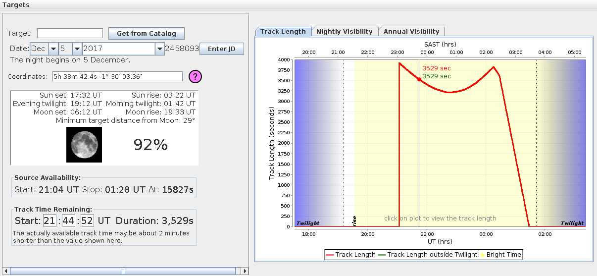
Figure 2.6. The SALT Visibility Calculator includes a tab displaying the available track length (the red curve) for a target.
2.6 Observing Blocks
All SALT observations are executed using Observing Blocks. These are defined as the minimum schedulable unit. A block must be allocated a single priority and have a single Moon brightness, seeing range, and transparency specification.
A block will consist of:
- One target;
- One acquisition (that is, telescope pointing and verification that the target is in the right position using snapshot images);
- One or more science procedures or instrument configurations.
This sequence of observations in the block plus all necessary overheads must fit within the target’s maximum available track time, inclusive of canonical overheads (900 seconds for MOS, 500 seconds for HRS and 600 seconds for any other instrument mode). It is thus useful to economise on the number of blocks to increase observing efficiency – but note the caveats below. Be aware that a target’s track time is less than or equal to its visibility time (Sec. 2.5). For a discussion on the ‘Too Tight Track’ (TTT) syndrome (where there is only a very short time window within which the SALT Astronomer can point to the target to obtain the track length required) please check our website: https://astronomers.salt.ac.za/software/visibility-calculator/.
A block will be executed under the specified weather conditions. If the weather conditions change within the hour, the block will be rejected and placed back in the queue for further attempts. If more than an hour has already been spent on a block, it will be accepted regardless (which argues for shorter block lengths and repeated blocks to reach the required exposure time).
A block will also be rejected and placed back in the queue if the data quality was compromised by technical difficulties with the telescope or instrument within the first hour of the block. (Note that the rejected data will still be available to the user).
Note that acquisition images are provided solely as a means of field identification and to allow positioning of the target(s). Acquisitions may thus be out of focus or otherwise unpalatable-looking: track time is valuable, and we do not want to waste time tweaking the acquisition images. The image quality will be refined before science data are taken. If focused SALTICAM images are required for science reasons, please add the relevant instrument configuration to the block. For RSS longslit observations, at least one in-focus SALTICAM slitview image will be provided.
Observing Blocks will be created in detail in Phase 2, but it is necessary to be aware of the basic principles when planning observations for Phase 1.
3. SALT Proposal Guide: Definitions and Procedures
Since SALT is a service mode telescope, the SALT proposal cycle consists of two phases:
- Phase 1 is the request for observing time and, after approval by the Time Allocation Committees (TACs),
- Phase 2 is the preparation of the approved observations.
The scientific justification of the program is the crux of Phase 1 and is evaluated by the relevant TAC, while SALT Astro Ops reviews the technical justification. Target information (where known), including numbers and lengths of visits to targets, is required already at the Phase 1 stage, as well as a high-level selection of an observing mode. The final detailed observing configurations of programs accepted by the TACs will then be submitted as part of Phase 2, and will be reviewed by the Astro Ops prior to being added to the observing queue. Changes to the target lists and other observation details may still be made at this stage within the constraints of the science goals in the proposal accepted by the TAC.
All proposals are created and submitted with the proposal and observation preparation tool (PIPT; see Sec 3.7 for details), both for Phase 1 and Phase 2. Phase 1 proposals may be submitted, edited, and re-submitted at any time before the deadline, as many times as needed. After the deadline, edits are no longer possible. Late submission policy is given in Sec 3.2.
Any questions during the submission phase should be emailed to salthelp@salt.ac.za. With the first submission of a proposal it will have been assigned a program code – in that case, that code must be provided in the subject line. See Sec. 3.7 for further details.
Items that need to be entered for the Phase 1 proposal include:
- Proposal type
- Required observation conditions
- Target details
- Time requested
- Instrument(s) and mode(s) required
- Description of program and justification
Once the TACs have approved proposals and allocated time according to priority class (see Sec 3.4), the Phase 2 proposals have to be completed adhering to these allocations (Sec 3.9). ToO alerts can be triggered at any time during the semester (Sec 3.9.1). Data can be retrieved either as raw data files or pipeline-reduced files (Sec 3.10). All PIs and Co-Is are invited to note our Publication and Acknowledgment Policy in Sec 3.11.
3.1 Who can apply?
Normal SALT proposals can only be submitted by astronomers who are members of a SALT consortium institution (Sec A.2), or are collaborating with such astronomers. Time can be requested from different SALT partner TACs according to the nature of the collaboration and it is entirely up to the PI and Co-Is to decide what fractions are requested from each TAC.
DDT proposals, on the other hand, can be submitted by any astronomer and no time will be charged to any SALT partner.
Anyone interested in purchasing time on SALT can contact the SALT Director, Dr. Encarni Romero Colmenero (erc@salt.ac.za), or the Chair of the SALT Board, Prof. Brian Chaboyer (brian.chaboyer@dartmouth.edu).
Time charging
At present, observing time is charged (that is, counted against the allocated time) on the basis of completion of requested observing blocks as they appear in the PIPT and SALT Web Manager.
3.2 Phase 1 late submission policy
- In general, no Phase 1 proposals will be accepted after the deadline specified in the Call for Proposals.
- If submission is prevented by technical issues (eg, problems with PIPT, network, etc), the PI should email a zipped version (.zip) of the proposal to SALT Astro Ops (sa@salt.ac.za) before the deadline, in which case this will be counted as a valid submission. SALT Astro Ops may, at their discretion, accept late submissions caused by technical difficulties at the receiving end.
- All other late submissions after the deadline will be flagged and forwarded to the relevant TAC(s). The PI will be requested to submit an appeal to the TAC(s) outlining the reasons for late submission. Acceptance of such proposals will be at the sole discretion of the relevant TAC(s).
Guidelines for the TAC regarding late submissions:
Late submissions that show no evidence of an attempt to submit or to make contact with Astro Ops before the deadline should be rejected, though the TAC may decide to accept the proposal following consideration of an appeal from the PI.
In any case, acceptance or rejection should be decided by the TAC(s) and communicated to SALT Astro Ops.
3.3 Proposal types
There are six proposal types which can be selected in the PIPT only when a new proposal is created:
- Science:
- Regular observing proposals (SCI): They follow regular Phase 1 / Phase 2 deadlines and procedures. Up to 150 hours may be requested.
- Long term (MLT): Identical to regular science proposals but request (and obtain) observing time for more than one semester.
- Large Science Proposal (LSP):
- Large Science Proposals request > 150 hours from one or more partners, which can be spread over a total of six semesters.
- Director’s Discretionary Time (DDT):
- DDT proposals may be submitted at any point via the PIPT, but they must be agreed upon with SALT (ddt@saao.ac.za) prior to submission. A total of 20h of DDT time is potentially available for 2026-1.
- Gravitational Wave program (GWP):
- GWP proposals may be submitted at any point via the PIPT. Please review our GW policy document beforehand for further information.
- Commissioning (COM):
- COM proposals intend to test new instruments, instrument modes or specific characteristics of the telescope/instrumentation. They have no science content, and usually only the instrument teams and SAs will submit these. In case of interest please email the SALT Astronomers (sa@salt.ac.za).
- Science Verification (SV) [not available this semester]:
- SV proposals intending to test the science capabilities of new or upgraded instruments, instrument modes or specific characteristics of the telescope/instrumentation. These are only available on a special Call for Science Verification proposals and must be agreed upon with SALT (sa@salt.ac.za) prior to submission.
Only the first two proposal types (SCI, MLT and LSP) require a Phase 1 submission, but the details required will depend on the type.
Multi-partner programs
If there are co-investigators from multiple partners in a single proposal, it is up to the Co-Is to divide the proposed time between the relevant partners, or request all of it from one partner. If a program applies for time from more than one partner, all the relevant TACs will receive the application and will allocate their time individually. It should be noted, however, that some TACs may look with disfavour on proposals from other partner institutions which request the majority of time from them if the respective Co-Is are minor players in the collaboration.
3.3.1 Science programs
Science proposals come in two flavours:
Regular programs (SCI)
Regular science proposals can request up to 150 hours and require a single semester to finish.
If you need to continue your program in the next semester, you may either submit a new proposal or submit a proposal progress report, as explained in the section on long-term programs (MLT). The functionality to submit a progress report became available in early January 2018.
Long-term programs (MLT)
Science proposals with up to 150 hours requested but which can or should be carried out over two or more semesters are called long-term programs. They will need to be specified as such in the Phase 1 proposal submission (the PIPT main page provides a box for Add time request for semester XXXX-X) and require a specific multi-semester justification.
These proposals, if approved for the current semester, will be automatically re-submitted for the next. However, a brief progress report is required for the follow-up semester(s) and must be submitted by the usual Phase 1 deadline. A form to enter this progress report is available on the proposal’s page in the Web Manager (https://www.salt.ac.za/wm/).
Please note that the TACs may re-adjust the time allocation before each semester. If no progress report is received, the TACs may decide not to continue the programme. If no time is allocated by the relevant TAC(s) in any given semester the proposal is no longer supported (i.e. the MLT status has been revoked). A new proposal will need to be submitted if more time is needed to complete the scientific goals.
3.3.2 Large Science Programs (LSP)
Science proposals requesting more than 150 hours from one or more SALT partners, which can be spread over a total of six semesters, are called Large Science programs. PIs considering submitting such a program should send an email to the Head of Astro Ops at saltastrohead@salt.ac.za with their intention to submit at least two weeks prior to the deadline to discuss overall feasibility and strategy.
LSP proposals will need to be specified as such in the Phase 1 proposal submission. The Phase 1 process is the same as for other proposals with the following exceptions:
- The PI will have a total of eight pages for the Scientific Justification and Technical Justification (using a special template file)
- The technical description is divided into two sections:
- Proposed observational setups and justification of the observing time required
- Management plan for reduction and publishing the data, including schedule
- For proposals with a large number of targets (greater than 20) or transient targets, the range and distribution of Right Ascension and Declinations should be supplied as part of the technical description, but all of the individual targets do not need to be entered.
LSP programs do not have any requirements on how the data are shared or how the time is distributed.
LSPs should propose only for commissioned modes of instruments which are listed in Sec 1.3.2. The proposal should include a strong justification for the total amount of time required. Science goals should be feasible. Programs with stringent conditions, poor target visibilities, or otherwise difficult observations will not be favoured currently. However, proposals for any type of science will be considered as long as the proposal is of very high scientific merit.
The criteria on which the LSPs will be judged are more stringent than for normal science proposals:
- Scientific merit, which is not limited to, but will include the overall importance of the science and particularly the probability that the observations will lead to rapid publications, the uniqueness of the project, and the overall impact of the project.
- Viability of the observations and most efficient use of the telescope under a range of conditions.
- Probability of success of the proposal including sufficient resources for the program.
- Management plan for the program, including how it will contribute to the SALT community.
As with all multi-partner programs, time will be allocated by the individual SALT partners specified in the proposal submission. In case of LSPs, though, Astro Ops will coordinate communication and discussion between the TACs before final allocations are made. Prior to the final allocation, comments from the TAC(s) will be distributed to the PIs of LSPs and the PIs will have a chance to reply or to adjust the proposal accordingly.
As for long-term proposals, approved LSP proposals will be automatically re-submitted for the next. However, a brief progress report is required for the follow-up semester(s) and must be submitted by the usual Phase 1 deadline. A form to enter this progress report is available on the proposal’s page in the Web Manager (https://www.salt.ac.za/wm/). Time and allocations are not guaranteed for future semesters, but require satisfactory progress being made on the proposals. TAC(s) may adjust their allocations according to how the proposal is progressing.
3.3.3 Director’s Discretionary Time (DDT) proposals
Only a Phase 2 proposal needs to be submitted for Director’s Discretionary Time (DDT) proposals (that is, the Phase 1 stage is not necessary). These do not need to follow the normal proposal cycle.
A total of 15-20 hours per semester of DDT time is available at present (see here for any possible changes or news). This time is not part of the SALT consortium time and thus DDT proposals can also be submitted by any astronomer including those that are not a member of one of the SALT consortium institutions (or collaborating with a member).
DDT programs must abide by the following rules:
- DDT proposals should be targeted for compelling relatively short observations which have potential for an immediate high impact result, i.e. a paper.
- DDT observations should ideally stand on their own, in terms of producing a compelling science result, rather than just being part of the longer term program (active or planned), though short "proof-of-concept" pilot programs that inform larger regular proposals may be considered.
- There should be good reasons for DDT observations to be done quickly, rather than being held over until the next proposal period (e.g. compelling ToO or opportunity of a quick high profile result).
- A free format (text or PDF or both) DDT proposal with sufficient motivation should be submitted to ddt@salt.ac.za and, having received an approval, should be submitted using the PIPT with “DDT” selected under “Proposal Type” which makes it automatically a Phase 2 submission. In urgent cases the proposer may submit the Phase 2 using PIPT at the same time as emailing the justification to ddt@salt.ac.za. Questions regarding DDT proposals can be also sent to salthelp@salt.ac.za. DDT proposals will be assessed by the Head of SALT Astronomy Operations and the SAAO Director who may consult with others within the SALT consortium regarding acceptability.
- All DDT observations with a SALT partner as PI or co-I become available to the entire SALT community within 6 months of them being taken. DDT observations from proposals with no SALT partner investigators become available to the entire SALT community immediately. In such a case, SALT will inform members of the SALT Board by email within 1 week of the observations being taken.
- Any DDT observations undertaken must be expeditiously analysed and the results of the program written up in a short report sent to SALT within 3 months of obtaining the observations. This report will be made available to the SALT Board. For positive science results, it is expected that the observations will lead to a quick scientific publication.
3.3.4 Commissioning (COM) proposals
Commissioning proposals are usually only submitted by members of the relevant instrument team and the SAs. Please contact sa@saao.ac.za if more information is required.
3.3.5 Science Verification (SV) proposals
Science Verification proposals are only available if a special Call for Science Verification proposals goes out once a new instrument or mode has become available and has been commissioned by the instrument team. This call will not follow the usual semester deadlines. The Call for Science Verification proposal document will contain all necessary information.
3.3.6 Shared-risk proposals
Shared-risk proposals for a new instrument or mode are called when a new instrument is expected to be available during the semester but the details of its actual performance are not known at the time of the call. Information will be made available as soon as it is known on a best effort basis as to the expected performance and updated once characterization takes place.
3.4 Proposal Priority classes
An individual observing program will consist of a number of Observing Blocks (Sec 2.6) of different targets which will be assigned a set of priorities by the relevant TAC(s). The priorities influence the likelihood of a given target being observed on a particular night and over a semester, see the Fig. 1.2 in Sec 1.2.
For the upcoming semester, the available science time will be allocated to the different priorities with 40% for P0+P1 time, 40% for P2 time, and 20% for P3 time with a factor 3 oversubscription rate for P3. These are applicable to both the regular science as well as the large science programs. The percentages are the same for each TAC and all observations are charged in the same manner (see Sec. 3.1).
Priority 0
Highest rated Targets of Opportunity (ToO) programs or time critical observations only. Once scheduled, and weather permitting, Priority 0 observations will have the highest chance of being observed at the time requested. Examples of such observations might include supernovae and other transient events, and rare periodic phenomena.
Any proposal can include time critical observations, but only those allocated a P0 priority will in general be observed in preference to other priority classes.
Note that P0 time is not permitted for non-time critical targets, P1 will be used instead.
Priority 1
Highest rated proposals or observing blocks, which, if scheduled, will have a high chance of being observed in a given night. Such targets will be the most scientifically compelling of all standard (i.e., P1 – P3) priority targets and completion of most P1 blocks in a given semester is expected. We expect to achieve at least 80% completion of P1 blocks, with the main problem being conflicting target distributions.
Priority 2
P2 programs or observing blocks are not as highly rated as P1 by the TACs, but are still considered to be compelling. P2 blocks will have a good chance (60%) of being completed in a given semester.
Priority 3
P3 programs or observing blocks are lowest priority science as assigned by the TACs, but still worthy of consideration. P3 proposals are deliberately oversubscribed by a factor of 3 in order to always have a full queue. If P3 blocks and programs are intelligently designed, that is, to be easy (short, loose constraints, wide RA-ranges with optional targets), dynamic scheduling will likely mean that more than the expected 20% will get observed.
Priority 4
This is a special priority class consisting of “filler” targets, to be done in marginal observing conditions (i.e. poor transparency or bad seeing) or to fill gaps in the observing queue. They would not need to be strictly 10-m class science, but deemed to be useful science nevertheless. P4 programs will not be charged. Contrary to the other priorities, P4 priorities are identified by the PI who should justify in the application (technical section) why their proposed programs should be considered P4 time (e.g. brightness, observing mode, allowable conditions, large pool of short observations). The TAC(s) will accept or reject the P4 proposals as they see fit. P4 programs will only be attempted if, at the duty SA’s discretion, there are no other viable P0 – P3 programs that can be attempted. Please note that P4 programs should ideally consist of short observing blocks, so that they may be slotted in as needed. As with the P3 programs, that is, if designed well, experience has shown that P4 programs can in fact get high completion fractions.
Note that SALT Astro Ops allows any TAC accepted program to add P4 blocks to their Phase 2 program free of charge, over and above their TAC time allocation – contact salthelp@salt.ac.za if you are interested.
3.5 Concept of “Optional Targets”
There are two types of SALT targets:
- Mandatory targets: These are all of the targets which the PI is expecting to observe if allocated the requested time.
- Optional targets: This is a pool of M optional targets from which the PI is requesting that any subset consisting of N targets can be observed within the allocated time. This target list is thus a super-set from which actual observations can be chosen, such that the total observing time of the eventual chosen targets equates to the total requested time of the proposal. The superset of targets (M) should be less than 5 × N, the number of targets actually likely to be observed given the requested time. The actual target choice will be dependent on the queue and chosen by the duty SA or scheduling algorithm. These pools can easily be defined in PIPT and they can also be built as monitoring pools where a wait-time can be defined after any of the pool members is observed.
We stress that the use of optional targets, especially when they have a wide RA-range, is extremely effective. You can significantly boost the chances of getting your program done if there is always one of your targets visible in the queue.
3.6 Observing constraints
The PIPT allows entry of observing constraints for the proposal. While individual constraints per target will only be needed for the Phase 2 proposal, the Phase 1 proposal requires information on the tightest observing constraints regarding seeing and cloud cover.
3.6.1 Definitions of Lunar illumination
PIs are free to specify any Lunar illumination fraction between 0% to 100% to define the maximum allowable lunar illumination for each observing block in Phase 1 proposals (under target information). In terms of often-used Dark, Gray, and Bright time terminology:
- Dark (50% of time): Illuminated Lunar fraction < 15% or Moon below horizon (Lunar phase angle > 135º)
- Gray (25% of time): Illuminated Lunar fraction = 15% – 85% (Lunar phase angle 45º – 135º)
- Bright (25% of time): Illuminated Lunar fraction > 85% (Lunar phase angle 0º – 45º)
- Any (100% of time): Lunar illumination fraction 0º – 100º, in which observations can be done in any Moon conditions
The PI is free to choose any fraction. For example, for a traditional Dark object the PI would use <15%, but if they were to specify a different fraction, e.g., <25% or <40%, they will get more flexibility in scheduling and thus a higher chance of completion. Note that the Bright targets, e.g. with <70% or <100% (i.e. the traditional Bright targets) will also be in the queue when the Moon is darker. PIs with equatorial targets please note that the Moon will likely be too close to the target for roughly ~50% of the traditional Bright time. During actual observations our scheduling tools will promote a dark block over a brighter block in dark time, but observations can be scheduled more efficiently when more blocks are available to choose from.
The PIPT for Phase 1 allows the specification of Lunar illumination for each target. Along with the proposal, the TACs will receive a summary on the approximate fractions of the proposed targets for the various Moon conditions. This information serves as a guideline only. The TACs will not specify a Moon condition for a program, they will only allocate time and priority. However, ideally all TAC partners should attempt to distribute their observing time allocations evenly over the range of Lunar phases.
In Phase 2, there will be an opportunity in the PIPT to also select a minimum angular Lunar distance; note that a default minimum angular Lunar distance of 30 degrees is already given, which can be changed if necessary.
PIs should also use the instrument simulators (Sec. 1.6) to ensure that overly demanding observing conditions are not requested unnecessarily.
3.6.2 Seeing conditions at Sutherland
The standard measure of atmospheric turbulence is the Fried parameter, r0. The SAAO (Sutherland) site uses an automated Differential Image Motion Monitor (DIMM) to measure this routinely and continuously. The blurring of an image at the focal plane of a large telescope, what we refer to as “seeing”, is derived from r0 using the standard model of atmospheric turbulence. It is a function of wavelength (λ) and airmass and the DIMM reports seeing using the convention of λ = 500 nm (essentially V-band) and airmass = 1.0. This is the value that is used to define observing conditions and make scheduling decisions.
Median zenithal V-band seeing, measured from the Sutherland DIMM at ground level, is ~1.5” (from measurements made over 2011–2021, see Table 3.1). Since the SALT visibility strip lies between 1.16 and 1.37 airmass this leads in principle to a factor of 1.1 to 1.2 degradation of seeing on average. This is broadly the case as can be seen in the actual distribution of seeing values shown in Fig. 3.1 for the 2021-2 semester, where DIMM values are compared with data taken by the SALT guider. Note that the active mirror alignment system (SAMS) was already installed for this period. This means that the actual SALT image quality (IQ) as measured by the instrument guiders is quite close to the zenithal seeing value, which is a drastic improvement from times before SAMS, that seasoned users of SALT should be aware of.
Table 3.1: Median zenithal seeing at Sutherland for past semesters
Semester | Median zenithal seeing |
2011-2 | 1.38” |
2012-1 | 1.56” |
2012-2 | 1.46” |
2013-1 | 1.47” |
2013-2 | 1.32” |
2014-1 | 1.52” |
2014-2 | 1.39” |
2015-1 | 1.43” |
2015-2 | 1.39” |
2016-1 | 1.49” |
2016-2 | 1.55” |
2017-1 | 1.50” |
2017-2 | 1.41” |
2018-1 | 1.59” |
2018-2 | 1.41” |
2019-1 | 1.52” |
2019-2 | 1.47” |
2020-1 | 1.67” |
2020-2 | 1.36” |
2021-1 | 1.53” |
2021-2 | 1.43” |
2022-1 | 1.46” |
2022-2 | 1.58” |

Figure 3.1: Seeing histograms from the SAAO DIMM and the SALT guider. The data are taken from the same period of time in 2025. Note that the guider data is corrected for the average airmass of SALT observations during this period. The PIs select their seeing restriction based on the intrinsic Zenith value and they now should expect a similar image quality delivered on the detector.
Table 3.2: Probabilities for a given seeing or better at the Sutherland site
Max Seeing | Probability |
1.25” | 26% |
1.5” | 50% |
2.0” | 82% |
2.5” | 93% |
3.0” | 97% |
Table 3.3: Expected image quality performance of SALT depending on seeing
DIMM zenith seeing | Seeing at average telescope airmass | FWHM | EE50 | EE80 |
1.0” | 1.2” | 1.4” | 1.6” | 2.6” |
1.5” | 1.7” | 1.8” | 2.0” | 3.3” |
2.0” | 2.3” | 2.4” | 2.7” | 4.2” |
As an aid to choose the most useful observing constraints, Table 3.2 shows the probability of having a given (or better) seeing, based on all the available seeing statistics. Table 3.3 indicates the expected image quality performance of SALT (in terms of the FWHM and enclosed energy diameters (50% and 80%) of the PSF for different DIMM seeing values (all V-band). The PSF is basically described by a modified Moffat function. The proposers should realise that it is the DIMM zenith seeing number that has to be inserted as “seeing” into the instrument simulator and used as the requested seeing, while the other numbers should be used to plan actual SNR. The simulators automatically correct the inserted seeing at zenith for airmass.
The results of a study looking into the causes of atmospheric turbulence above the Sutherland observing site are presented in Catala et al. 2013.
3.6.3. Definition of cloud cover conditions
The cloud cover conditions are
- Clear
- Thin Cloud
- Thick Cloud
We define thin cloud to range between occasional thin clouds passing over (e.g. partly clear) to consistent all sky thin cirrus. Thick cloud corresponds to a moderate to heavy extinction and when guidance is often interrupted due to the guide stars being partially or fully obscured for a good portion of the track. Short exposures of bright stars are best suited to thick cloud conditions.
3.7 Phase 1 proposal preparation and submission
All investigators (PI and Co-Is) on a SALT proposal must have an account on the SALT server before the proposal can be submitted. This can be created by means of the Web Manager by pointing a browser to https://www.salt.ac.za/wm/Register/. After a successful registration, a confirmation email is sent, which includes instructions for validating the chosen email address.
Once an account has been created, the Web Manager can be used to view one's proposals (including unsubmitted ones) and to update one's contact details.
All proposals are created and submitted with the proposal and observation preparation tool (PIPT), both for Phase 1 and 2. This is a stand-alone application requiring Java 1.8 or higher. While the Open JDK may work, using the Java environment provided by Oracle is strongly recommended. (http://www.oracle.com/technetwork/java/index.html). The PIPT itself can be downloaded from http://astronomers.salt.ac.za/software/. A manual for the PIPT is available both as html and pdf.
The scientific and technical justification needs to be generated from a Word/Latex template, which can be downloaded from:
http://astronomers.salt.ac.za/proposals/proposal-templates/
Some common questions and issues are addressed below; however, a more complete, live, and frequently updated online FAQ is available at:
http://astronomers.salt.ac.za/proposals/faq/
In the PIPT, new proposals can be created with the File > New Proposal menu item. The PIPT will ask which type of proposal to create (see Sec. 3.3). Note that only a Science or Large Science proposal will be forwarded to the TAC (see Sec. 3.3 for details).
The main items to be entered in the PIPT for Phase 1 are:
- investigator details
- proposal type (Sec 3.3)
- required observing conditions (Sec 3.6)
- target details (if known, cf. Sec 3.5)
- the time requested
- instrument(s) and mode(s) required, including saved Instrument Simulator setups
- brief report on previous SALT proposals by the same PI (optional for some partners) and a list of SALT-related publications
- a brief description for the general public
- basic description of program and technical justification (including observing constraints)
- scientific justification & description (optional for some partners)
All but the last two bullet points are entered in the respective boxes in the PIPT form, while the last two items must be included in the form as a PDF. This PDF file is limited to four pages in length (eight pages for Large Science Proposals). The PDF must be generated using the latest version of one of the templates provided (in Word, OpenOffice, or LaTeX format). These can be downloaded from:
http://astronomers.salt.ac.za/proposals/proposal-templates/
Note that Large Science Proposals use a different template from the rest of the proposal types. You have to use the template for the current semester; you cannot reuse templates from the previous semesters. Word limits quoted in the template should be considered guidelines as long as the total proposal length is less than four (eight for LSP) pages including references and figures.
SALT observing programs distinguish between the Principal Investigator (PI) and a Principal Contact (PC). The latter will be the actual liaison between the proposing team and the SALT team, do the Phase 2 proposal preparation and submission, receive the data etc. For large collaborations it may be desirable to set up a group emailing address so that several people can share in. Note that only the PC will receive communication through the Web Manager regarding clarifications on the proposal, questions and information during observing and notifications when the data becomes available.
Targets and instrument configurations have to be defined for a Phase 1 proposal. These may be added by right-clicking on a node in the navigation tree (on the left). Similarly, adding and removing content from a table can be accomplished by right-clicking on the table.
Warnings should be taken very seriously, as they often indicate a serious flaw in the proposal. In most cases, submission is only possible once the problem has been fixed. An explanation is displayed by clicking on the little warning sign next to the problematic input.
More details about the PIPT can be found in the manual, which is available both as html and pdf.
Before a proposal is submitted, it should be validated with the menu item Proposal > Validate. If the validation fails, this usually means that some required input is missing. Note that valid Phase 1 proposals may be submitted, edited, and re-submitted at any time before the deadline, as many times as needed. It is recommended to re-submit frequently to ensure that the final submission goes smoothly and does not cause unnecessary delays in the final submission.
After the first successful submission of a proposal, a confirmation email with the proposal code is sent to all investigators. This proposal code uniquely identifies the proposal, and it should be quoted in the subject line of any email query related to the proposal. The proposal code is also added to the proposal itself, so that resubmissions do not generate new proposals in the database. It is a good idea to double-check that the correct proposal code is shown in a submitted proposal. Confirmation emails for re-submissions are only sent to the investigator re-submitting the proposal.
When logging in to the Web Manager, a list of the user's proposals is shown. Clicking on any of the proposals leads to a page with the proposal details, which may be used to check a submitted or resubmitted proposal. However, it may take a few minutes before the content is fully visible after submission (especially finding charts). It is also possible to import a proposal in the PIPT (using at the top menu bar: either File -> Import from Zip file or Online -> Import from Server), e.g., for a Co-I to access a current proposal, or to recover an old proposal. Note that when a proposal of the same code already exists on the user’s computer, the version on the computer will be replaced with the imported one (the user will be warned beforehand).
In addition to the Web Manager and the PIPT, a Visibility Calculator and Simulator Tools are supplied for SALTICAM, RSS and HRS, which can be used to plan the required instrument setup and the necessary exposure time (see Sec 1.6 for all downloads). They also require Java 1.8. These Simulators allow the user to define a target spectrum and an instrument configuration, and to calculate the signal-to-noise ratio expected for these. They are always updated to the latest information regarding sensitivity, throughput and other instrumental constraints so please make sure you have the latest version. It should be noted that the Simulators do not take any overheads into account when calculating the signal-to-noise ratio.
The PIs should be aware that the wavelength ranges predicted by the RSS Simulator currently may have inaccuracies up to +/– 2 nm.
Simulated setups can be saved from the Simulator Tools, and these saved setups should be attached to a Phase 1 proposal in the PIPT for use in the technical reviews (under the Instrument Configuration nodes). The technical justification may refer to these attached instrument setups.
3.8 The procedure between the two proposal phases
All Phase 1 proposals will first be directed to the SALT Astronomy Operations team for a technical feasibility assessment. Comments on technical feasibility will be forwarded to the individual TACs of the SALT consortium. The TACs will then allocate time to successful proposals in various priority classes. The minimum time allocation for a successful proposal will be 900 seconds per priority.
In cases where only a small fraction of the time requested for a multi-partner proposal is awarded by the relevant TACs, the Head of Astronomy Operations will engage with the relevant TAC Chairs to ensure that the allocation can actually result in a meaningful program.
After the full TAC review and time allocation process has been completed for all partners, PIs will be notified of the outcome. These notifications mark the start of the Phase 2 submission period.
3.9 Phase 2 proposal preparation and submission
The notifications of the TAC outcome mark the start of the Phase 2 submission period, during which the detailed observing blocks must be submitted by the PCs to SALT operations using the PIPT. Changes to the target lists and other observation details may still be made during this stage within the constraints of the science approved by the TAC. Any other changes need the approval of the Head of Astronomy Operations who may refer the request to the relevant TACs.
Proposals with Phase 2 material submitted early may be considered for observations even before the new semester observations officially commence, depending on the status of the queue of the previous semester projects. There is a strict deadline for the Phase 2 submission phase (see Sec. 1.5), which is crucial for planning the schedule for the semester. We cannot guarantee that programs submitted after the Phase 2 deadline will be included in the observing queue. If there are problems causing delays please be in contact with SALT Operations before the deadline.
For a Phase 2 proposal, the PIPT will ensure that:
- It does not require more observing time than allocated by the TAC;
- It does not contain any Observing Blocks with sky conditions tighter than those requested during Phase 1 and approved by the TACs. Conditions may be relaxed, however.
ToO programs that do not yet have targets available should submit dummy block(s) so their configurations can be reviewed. For normal proposals, all targets must be submitted at the deadline, but updates (within the constraints of the approved science) may be supplied throughout the semester if required.
All accepted SALT proposals will be assigned a Liaison SALT Astronomer (LSA) who will be the main point of contact between the PI and SALT Astro Ops. Communications regarding the completion of the Phase 2 proposal, the status of the proposal and issues regarding the observations and data should be communicated with the LSA in the first instance. Do not forget to quote the proposal code in the subject line of any email communication.
3.9.1 ToO alerts
For activation of ToO programs, PIs or PCs should communicate their request to salthelp@salt.ac.za.
3.9.2 Submitting via a Python script
The PyAstroSALT library provides a wrapper around SALT’s Application Programming Interface (API). In particular, it offers a function for submitting a proposal. At the moment, the proposal must be supplied as a zip file (as you would get it when exporting from the PIPT). PyAstroSALT should be considered experimental, and we strongly encourage PIs to contact SALT Astro Ops before using it. Phase 1 submissions should only be done via the PIPT.
3.10 Data distribution and reduction
The PC of the proposal will receive an email with download instructions as soon as the data are ready to be downloaded, generally the morning after the data have been taken. This includes the raw data, processed data (see Sec. 3.10.2), and documentation including the night log. Due to disk space constraints, the data will remain on our FTP server only for two weeks. However, the PC and co-Is may request a dataset again. Please visit the Web Manager and load the relevant proposal. The data can be requested in the last column from the table listing the observations taken for the proposal. The relevant data will then be placed in the public FTP server for another two weeks, and the PC will be notified by automated email when the data are ready to be retrieved. This should happen fairly quickly, so please contact us at salthelp@salt.ac.za if you do not receive the email notification within 24 hours.
Standard star calibrations taken with the same setting as the proposal may also be requested using the Web Manager from a button located at the bottom of the table listing all the observations taken for the proposal.
The PI has two options for data distributions: Normal and Fast:
- For “Normal” data distribution, the PI will receive an email once the data have passed through the pipeline in Cape Town. This will typically be within 12 hours of the observations, but may be up to one week later.
- For “Fast” data distribution, the raw data will be made immediately available along with any quicklook products. Once the first observation has been taken for the proposal during a night, the PC will be notified that observations are being made for their proposal. Due to limits on bandwidth and data processing, we ask that only proposals that would truly benefit from this high response time select this option.
A searchable data archive was launched in July 2020 (https://ssda.saao.ac.za/). Details on the proprietary period for various data sets can be found in the next section.
3.10.1 Data proprietary period
Data will become publicly available in the SALT Data Archive (https://ssda.saao.ac.za/) after the following periods, counting from the end of the last semester that datasets were taken for the relevant proposal:
- Science proposals: 36 months, or 24 months if South Africa has allocated time
- Director's Discretionary Time proposals: 6 months
- Gravitational wave proposals: 0 months, data only available to SALT partners
- Commissioning proposals: 36 months
- Performance verification proposals: 12 months
Science proposals with no South African time allocation may have the proprietary period extended. For all other proposals, you may request an extension of the proprietary period. Both can be done from the relevant proposal's page in the Web Manager.
3.10.2 SALT pipeline data reduction
The SALT data reduction pipeline was last upgraded on 1 August 2024. It processes the previous night’s data at 10:30 am (SAST) each day. The pipeline will pre-process the data, reduce observations from each of the different instruments, assess the data quality of the observations, and distribute the observations to the investigators.
The primary data reduction pipeline will process all observations for basic CCD reductions. This includes bias subtraction, gain correction, cross-talk correction, and mosaicking the different CCD chips. For HRS data (all modes not including High Stability), the secondary data reduction pipeline will also wavelength calibrate and extract the spectra. For RSS longslit data, the secondary data reduction pipeline will apply cosmic ray removal and wavelength calibration.
All of the raw and reduced data will be made available in the SALT FTP directory for the user. This is accessible at ftp://saltdata.salt.ac.za, using the user’s login for the Web Manager, as a zipped tarball file. In addition to the raw and reduced data, the astronomers log, environmental information, and other documentation is also provided in the directory.
3.10.3 SALT data reduction user packages
As of 1 August 2024 all SALT data is processed by the updated Python-based SALT data reduction pipeline (see Kotze et al. 2025). This includes a Python-based automated RSS data reduction pipeline, whose documentation and installation instructions can be found here: https://astronomers.salt.ac.za/software/rss-pipeline/. All RSS longslit data is reduced using the pipeline and the data products are sent to users. Please note that the pipeline may also flat field RSS data. This functionality is currently not operating as intended, and is being investigated, in the meantime users are advised to use the pipeline software to re-reduce the data without applying the flat fielding. RSS spectropolarimetry data is also reduced automatically by the polsalt pipeline (see below), and HRS data is reduced by the MIDAS pipeline (see below). The RSS Slitmask IFU pipeline is under development, but there are IRAF based data reduction recipes provided in the documentation. Please cite and include links to the appropriate software used in your data reduction and analysis.
The PySALT user package was the primary reduction and analysis software package for the SALT telescope. It is no longer used in the primary reduction pipeline and it is, unfortunately, no longer being developed. It can either be downloaded from http://astronomers.salt.ac.za/software/ or installed directly via Docker: https://astronomers.salt.ac.za/software/pysalt-documentation/. These tools include basic data reductions for RSS and SALTICAM in both imaging, spectroscopic, and slot modes. Basic analysis software for slot mode data is also provided. These tools are primarily written in python/PyRAF with some additional IRAF code.
Documentation is available on the http://sciencewiki.salt.ac.za/index.php/PySALT, in user manuals, and also provided within the package itself. PySALT Data Tutorials can be found on the SALT sciencewiki pages at https://sciencewiki.salt.ac.za/index.php/PySALT_Data_Tutorials. A script for fully reducing long slit and MOS data is also available here: https://github.com/crawfordsm/zsalt .
SALT RSS data have also been reduced using the IRAF reduction package. A recipe on how to reduce longslit spectra can be found on the sciencewiki at https://sciencewiki.salt.ac.za/index.php/Long_Slit_Reduction_Recipe. A more comprehensive report can be found in http://www.saao.ac.za/~akniazev/pub/SALT_Long_slit.pdf. Furthermore, a recipe on using a combination of packages IRAF, PyRAF and other packages can be found in http://www.saao.ac.za/~akniazev/pub/RAIL_README.pdf.
You may contact salthelp@salt.ac.za for assistance or advice with longslit spectra reductions, especially if you have a large number of spectra.
Analysis software for RSS spectro-polarimetry is available at https://github.com/saltastro/polsalt.
For the reduction of SALT HRS data there is currently one package available: MIDAS (Kniazev et al. 2016a, 2016b).
3.11 Publication and acknowledgment policy
Publications
Please notify salthelp@salt.ac.za of any publication made using SALT data including reviewed papers and conference proceedings.
Science paper acknowledgements
All science papers that include SALT data which are submitted for publication in refereed science journals must include the following words of acknowledgment:
“All/some [choose which is appropriate] of the observations reported in this paper were obtained with the Southern African Large Telescope (SALT) under program(s) [insert Proposal Code(s)].”
We recommend that the Principle Investigator is also mentioned after the Proposal Code. In addition, for papers which predominantly based on SALT data, a footnote symbol should appear after the paper title*, and the following text should be written as a footnote:
*based on observations made with the Southern African Large Telescope (SALT)
If possible, please also include the Proposal Code and Principle Investigator in the body of the paper when describing observations.
If you use data reduced using the PySALT software, please provide a link to http://pysalt.salt.ac.za/ and cite the following paper:
Crawford, S.M., Still, M., Schellart, P., Balona, L., Buckley, D.A.H., Gulbis, A.A.S., Kniazev, A., Kotze, M., Loaring, N., Nordsieck, K.H., Pickering, T.E., Potter, S., Romero Colmenero, E., Vaisanen, P., Williams, T., Zietsman, E., 2010. PySALT: the SALT Science Pipeline. SPIE Astronomical Instrumentation, 7737-82
References
In addition, the following papers provide a description of the telescope and instruments:
SALT:
Buckley, D.A.H., Swart, G.P., & Meiring, J.G. 2006, Proc. SPIE 6267, 62670Z
RSS:
Burgh, E. B., Nordsieck, K. H., Kobulnicky, H. A., et al. 2003, Proc. SPIE, 4841, 1463
Kobulnicky, H. A., Nordsieck, K. H., Burgh, E. B., et al. 2003, Proc. SPIE, 4841, 1634
RSS FP:
Rangwala, N., Williams, T. B., Pietraszewski, C., & Joseph, C.L. 2008, AJ, 135, 1825
SALTICAM:
O'Donoghue, D. et al. 2006, MNRAS, 372, 151
SALT-HRS:
Barnes, S.I., et al 2008, Proc. SPIE 7014, 70140K
Bramall, D.G., et al 2010, Proc. SPIE 7735, 77354F
Bramall, D.G., et al 2012, Proc. SPIE 8446, 84460A
4. Telescope Performance and Observing Constraints
Section 2 explained the basic concepts to understand when planning observations with a telescope like SALT, especially regarding the track times, the visibility of objects and the effect of the moving pupil for absolute (spectro)photometry. This section will define the characteristics and performance of the telescope and general, instrument-independent issues.
SALT is situated at the South African Astronomical Observatory (SAAO) field station near the small town of Sutherland, in the Northern Cape province, about 400 km from Cape Town. Its coordinates are: Latitude: -32 22 46, Longitude: 20 48 38.5 E, and elevation: 1798 m.
The SALT mirror comprises 91 hexagonal segments figured to have spherical surfaces with a radius of curvature of 26.165 m. When all segments are pointing to a common focus, they act as a 10-m spherical mirror. The effective area for a given observation, however, is more likely that of a 7─9-m telescope for two reasons: (i) only a subsection of the full mirror is seen by the tracker (the ‘pupil’, see Sec. 2.3 for more details), and (b) since the instruments are placed in the prime focus, some of the light is blocked by the payload. Both effects vary with the tracker position and thus during an observation. See Sec. 4.4 for details.
4.1 Image quality (IQ)
Active control of the mirror segments with new mirror edge sensors, called SALT Array Management System (SAMS), became operational in early 2016 with excellent results (see Sec. A.3). Images are now stable throughout the night over large temperature gradients, and observations are only limited by intrinsic seeing and, occasionally, dome seeing. It is therefore now feasible to request 1.5” seeing for faint and challenging targets; good results for e.g. high-redshift point source spectroscopy have been demonstrated. Please note that sub-arcsec conditions are extremely rare.
4.2 Vignetting
There is strong vignetting of the 8’ x 8’ Field-of-View, as shown in Fig. 4.1. Objects observed more than 2 arcmin from the centre of the field receive up to 10% less light (depending on the instrument used), and this needs to be taken into account when planning to make use of targets over the full field of view (this is not incorporated into the simulators). These numbers are greater than the specification and are still under investigation.
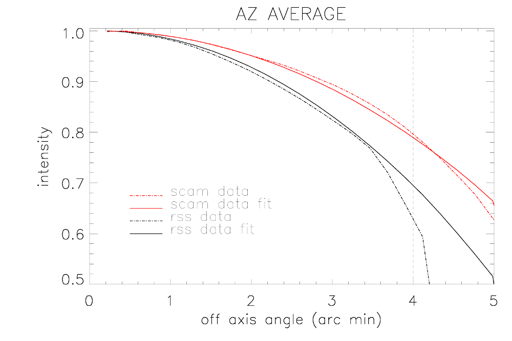
Figure 4.1: Vignetting of the FOV with RSS and SALTICAM.
4.3 Throughput
The primary mirror is kept clean by regular (every week or two) cleaning with high-pressure CO2, and individual segments are normally taken out for washing and re-coating in a cycle of nominally about 12 months. This has been standard practice since 2012. Throughput of the telescope is routinely monitored using SALTICAM (since there are no significant optics in this instrument, these values can be thought of as an approximation of the telescope throughput) by measuring standard stars with the primary mirror in “burst mode” where each segment forms an independent image of the star. Figure 4.2 shows the yearly measurements, corrected for the estimated total efficiency of the instrument (filters, CCD, foreoptics) and the atmosphere. Only the 7–10 best quality mirror segments are used to derive these numbers, while the values implemented in the Simulator are taken to be 15–20% worse to describe a typical track across mirror segments that are in different stages of cleanliness. For comparison, the system specification is shown as well (dashed black line).
The telescope throughput has increased significantly from before to after the 2020 shutdown, being better than the expected throughput in the red part of the spectrum, but not yet at blue and intermediate wavelengths. The August 2022 results indicate that the throughput has decreased dramatically. This has been attributed to a significant drop in mirror reflectivity due to struggles with the mirror coating plant. The mirror coating process has since been revised and is also now performed more frequently, which has led to an improvement in the throughput. We should also mention that a new ADC was installed in September 2022. This could also have contributed to the improved results, although we cannot confirm how much. To calculate the telescope throughput, we assume a fixed SALTICAM throughput. Since this time around all three systems (the telescope’s SAC, SALTICAM optics and RSS optics) were cleaned, it is not possible to establish where the improvements are. There still appears to be some blue loss in SALTICAM. We suspect an ageing SAC to be the largest contributor to the slightly less than optimal system throughput, but a full recoating is not likely for a while.
As part of the shutdown preparations in 2025, a new throughput measurement was taken on 23 March 2025, and the reduction of this dataset has revealed a concerning issue: a significant drop in telescope throughput — on average 18% lower than the last measurement from October 2024.
The SAC mirrors have advanced multi-layer coatings, expected to last the lifetime of the telescope, and the SAC was never designed for easy access or long-term servicing beyond dust cleaning. However, after 20 years of exposure, one of the coating layers in one of the mirrors has now failed internally, and another mirror shows early signs of degradation. This is not something that could have been prevented. This deterioration now significantly impacts sensitivity, particularly for fainter targets.
Subsequent throughput measurements taken after the 2025 shutdown, one in June 2025, one in September 2025 and another in December 2025 indicate that the previous decrease in throughput has stabilised, with no further throughput loss detected.
In the interim, proposers are encouraged to factor in the reduced throughput when planning observations. The SALT instrument simulators have been updated to reflect the current throughput and will continue to be maintained accordingly.

Figure 4.2: Current and historical telescope (that is, SALTICAM) throughput values for different wavelengths (in micrometres). The most recent values are indicated with the brown stars. Measurements correspond to the 7–10 best quality mirror segments.
[Note: This section is for the old RSS detector and is kept here for completeness until the throughput is quantified with the new detector.] The RSS instrument-specific throughput had been significantly reduced over all wavelengths since the re-commissioning of the instrument in 2011. A major overhaul of RSS took place in September and October of 2014 during which many of the optics were cleaned and optical coupling fluids in the collimator were replaced. This resulted in approximately 40% increase in RSS throughput (and more in the blue part of the spectrum) judged from both pre-installation laser measurements and on-sky standard star measurements. Additional causes of poor throughput were attributed to several degraded coatings, though the fixing of these is now on-hold due to lack of funding. A new optical service was done in August 2016 which recovered the slowly deteriorating RSS efficiency (by about 10%) to the clean 2014 values. It is now planned that RSS will undergo a routine optics clean every 24 months or so.
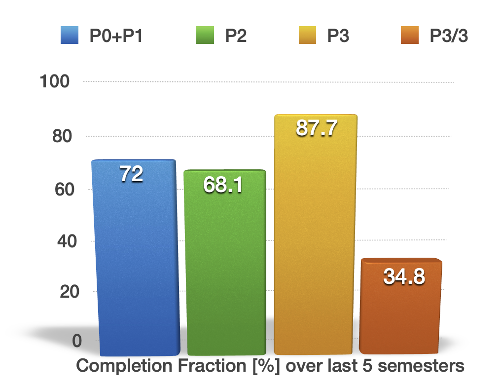
Figure 4.3: Current and historical RSS + telescope throughput values for different wavelengths (in micrometres). The most recent values are indicated with the yellow points.
The RSS + telescope throughput increased significantly after the shutdown in 2020 (Fig. 4.3). It must be again noted, however, that since both SALTICAM and the SAC were cleaned but SALTICAM has been assumed to be constant, the increases in throughput due to SALTICAM are now assigned to RSS + telescope. There has been a steady decrease in the throughput since 2021. As mentioned above, this has been attributed to the SAC mirror coatings failing. The latest results (indicated by the yellow stars) indicate that the previous decrease in throughput has stabilised, with no further throughput loss detected.
We stress that the current throughput values as discussed above are incorporated into the latest instrument Simulators which should be used for planning your program. Any noticeable changes will be immediately incorporated into the simulators, and, where necessary, the community will be informed. Finally, note that while the atmosphere has been corrected in Fig. 4.2, its effect is included in the Simulator tools and can be adjusted therein.
4.4 Collecting area
The nominal collecting area of the primary mirror with a central track after all obscurations are subtracted, is ~55 m2, decreasing to ~40 m2 for extreme off-axis tracker positions. This means that SALT is equivalent to between a ~7 to 9 m diameter conventional telescope depending on the pupil (Sec 2.3).
The current default collecting area in the instrument Simulators is set to 46 m2 (or approximately 53 fully illuminated segments) – this corresponds to experimentally derived averages of visible pupil area with tracker obscuration over a full track, and also makes allowance for the fact that the throughput calculations referred to above are normally done for a dozen or so best-quality segments. The collecting area is an adjustable parameter in the Simulators, but it should only be changed with caution.
5. SALT Calibration Plan
SALT calibration data are divided into four categories:
- Default calibration (DC):
- will be produced for every observable night
- will be produced without PI request
- PIs will not be charged
- will be done during day or morning time, possibly twilight and nighttime
- Library calibration (LC):
- will be produced at some regular interval, not every observable night
- will be produced without PI request
- PIs will not be charged
- will be done during daytime, possibly twilight and nighttime
- User-requested charged calibrations (UCC):
- will be produced by PI request
- will be done during nighttime
- PI will be charged
- User-requested non-charged calibrations (UNC):
- will be produced by PI request
- will be done during daytime and/or twilight
- PI will not be charged
Please see the instrument-specific sections for the current semester calibration plans.
6. SALTICAM
6.1 Current status
SALTICAM is available for this semester. There is a new website that lists the installed SALTICAM filters live and should be used for the Phase 2 proposal preparations: http://astronomers.salt.ac.za/status/.
Although guiding with SALTICAM is possible, several of its features make it impractical for many applications (see Sec. 6.9). Overall, we suggest limiting SALTICAM exposure times to approximately 120 seconds with open-loop tracking. For longer exposures we strongly suggest using RSS. If SALTICAM filters are needed for RSS imaging, please contact the SALT Helpdesk well in advance to check the feasibility of this and to ensure that there is enough time to transfer them to RSS. Frame Transfer and Slotmode imaging are no longer offered using SALTICAM, but these modes are offered with RSS.
6.2 Characteristics and performance
SALTICAM is a UV–Visible imaging and acquisition camera, capable of high time resolution imaging (down to 0.05 seconds). It consists of two E2V 44–82 CCDs (2048 x 4102 x 15 µm pixels), which are physically separated by a 1.5 mm gap and are read out by four amplifiers. SALTICAM is at prime focus; however, it is fed by a fold mirror and has a reduced focal ratio of f/2. The result is a nearly 10-arcmin diameter field of view, with the central 8-arcmin diameter portion being used for science and the outer annulus for guide stars as shown in Fig. 6.1 (but see Sec. 4.2 on vignetting). The plate scale is 0.138 arcseconds per unbinned pixel. A wide range of filters are available, spanning the wavelength range 320 – 950 nm. Due to the variable pupil, the best achievable photometric accuracy is 0.05 mag. This accuracy can only be reached for stellar objects by using dithering (see Sec 6.8).
More details on this instrument can be found in the appendix (Sec A.5). A simulator that uses target characteristics and a detector configuration to return count rates, signal-to-noise ratios, pixel saturation, and readout times can be downloaded from https://astronomers.salt.ac.za/software/#SALTICAM.
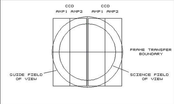
Figure 6.1: SALTICAM full layout. For details see Sec. A.5.
6.3 Readout speed and gain settings
There are four possible combinations for readout speed and gain settings, returning gain values between 1.0 and 4.5 electrons/ADU with readout noise of either 3.3 or 5 electrons per pixel (Tables 6.1 and 6.2, respectively). The dark current is typically less than 1 electron per pixel per hour. The full well depth is on the order of 170 000 electrons. Pixel pre-binning from 1x1 to 9x9 (independent in each direction) and up to ten subframe windows can be selected. The readout times for full frame with 2x2 binning are given in Table 6.2.
Readout Setting | Gain Setting | Actual e-/ADU |
Fast | Faint | 1.55 |
Fast | Bright | 4.5 |
Slow | Faint | 1.0 |
Slow | Bright | 2.5 |
Table 6.1: Gains for the four different readout modes selectable on SALTICAM.
Detector Mode | Pre-bin | RO mode | RO Noise (e-/pix) | Total Readout Time (sec)* |
Full Frame | 2x2 | Slow | 3.3 | 21 |
Full Frame | 2x2 | Fast | 5.0 | 14 |
Table 6.2: Readout (RO) times of SALTICAM for the 2x2 binning. Refer to Sec A.5 for times of other binnings. *Inclusive of CCD readout, disk writes, and software overheads.
6.4 Available instrument modes
The standard mode of operation is normal imaging (full-frame readout). Please note that frame transfer (half-frame readout) and slot mode (144-row readout) are no longer offered on SCAM. However, these modes remain accessible on RSS. Specific characteristics for the normal imaging mode, as well as the specialised modes of non-sidereal tracking and drift scanning, are discussed below. Note that absolute photometry is not possible with SALTICAM alone because of the moving pupil (see Sec 6.6). All the sub-framing, preamplifier binning, gain, and filter options listed for SALTICAM are available in all instrument modes.
6.4.1 Normal imaging
Normal imaging is the basic, full-frame SALTICAM mode, which also serves as the acquisition mode for spectroscopic observations.
6.5 Filters
SALTICAM has an eight-position filter magazine. Available filters are listed in Table 6.4. The transmission curves can be viewed in the PIPT.
The SALTICAM CCDs were optimised for visible and near UV imaging, thus no effort was made to minimise fringing at near IR wavelengths. We have not yet quantified the amplitude of fringing in all filters. We have observed fringes with an amplitude of ∼10% peak-to-trough for red, narrow-band filters such as z’. Fringing is not an issue for broadband filters or those at the shorter end of the wavelength range.
Type | Name |
Johnson-Cousins | U, B, V, R, I |
Sloan | u’, g’, r’, i’, z’ |
Strömgren | u, b, v, y, H-β wide, H-β narrow, SRE1, SRE2, SRE3, SRE4, Clear |
Other | H-α (zero redshift) 380-nm (FWHM 40Å) neutral density |
Table 6.4: SALTICAM filters.
6.6 Photometric accuracy and flat-fielding
NOTE: the text below presents the ideal, expected situation. Flat-fielding in particular remains an unsolved issue, and even relative photometry within the SALTICAM FoV has not been achieved to much better than 5% accuracy (see Sec. 6.10.1 on calibrations for more details).
The moving pupil, inherent to the basic operation of SALT, presents special problems for doing photometry with SALTICAM. While it is true that if the tracker position is known at all times, the fraction of the primary mirror within the pupil can be calculated (including gaps between mirrors) and the photometric "response" function of the telescope can be worked out. However, this assumes equal reflectivity for all mirrors; clearly this will not be true and furthermore it will be variable as the cycle of mirror recoating runs. (Typically, at least one and possibly two segments per week will be re-coated).
Due to the inherent uncertainty in measuring mirror reflectivities, it is highly challenging to provide calibrations sufficient to estimate the response function to an accuracy of 1% or better across all tracker positions. So those carrying out photometry with SALTICAM should bear in mind:
- Relative photometry within the 8-arcmin science field is unaffected by the pupil/primary mirror mismatch because the mismatch impacts all field angles equally. While the SAC introduces spatially variable vignetting across the field, this effect is constant in time; the instrument team will provide calibrations to correct for this during data reduction. Consequently, programs requiring relative photometry of point sources or extended objects will not be compromised. For variability monitoring, the target must be referenced to one or more stable comparison stars within the same field.
- Absolute photometry with SALTICAM is not possible because the pupil/primary mirror mismatch varies. Instead, absolute calibration requires referencing the SALTICAM data to known magnitudes of at least one (and preferably several) point sources within the field. These reference magnitudes must be in the same filter system and can be obtained either from existing catalogs or through supporting observations on another telescope.
- Most accurate absolute photometry, especially in the U-band, will require knowing the colour transformation equations for the SALTICAM filter system. Determining these is not a trivial task and will require observations of a cluster of stars with known and reliable photometry.
For more information on SALTICAM photometry and flat-fielding, see these two documents (you will need your Web Manager login credentials to access): https://sciencewiki.salt.ac.za/index.php/File:Salticam-phot-nov2011.pdf and https://sciencewiki.salt.ac.za/images_sciencewiki.salt.ac.za/1/1b/SCAM_obs.pdf
6.7 Sensitivity
All SALTICAM sensitivity calculations for planning observations should be done with the latest version of the SALTICAM Simulator tool (see http://astronomers.salt.ac.za/software/). The tool uses throughput values derived from observations of Sloan comparison fields and primary mirror tests conducted in “burst mode” (where each segment forms an independent stellar image). These baseline values are then extrapolated to represent a typical pupil during a track (see Sec 4.3 for details). We have directly verified count rates up to about 5-minute exposures and these behave as expected. Longer integrations are not practical due to the difficulties with auto-guiding (see Sec. 6.9) and SALT’s current open-loop tracking performance.
To achieve the deepest SALTICAM imaging, observers should ideally co-add short (~2-minute), dithered exposures (see below). Recent programs using this strategy have successfully detected targets down to g = 24.7 mag and r = 24.1 mag. However, achieving theoretical signal-to-noise scaling in stacked images depends heavily on flat-field quality (see Sec. 6.6) and point spread function (PSF) stability over tens of minutes. Although PSF stability has improved significantly with the recent introduction of the active mirror alignment system (SAMS), the exact sensitivity limits of longer stacked sequences have not yet been fully characterised. Therefore, PIs are urged to be conservative when estimating the expected depth of their observations.
6.8 Dithering
As previously noted, because the moving pupil complicates flat-fielding, dithered observations yield the best photometric results across the field of view.
The most productive dithering schemes will depend on the science goal and size of science targets. For Phase 2, a user-selectable dithering pattern is supported in the PIPT – please see our website for a description of the available dither patterns: http://astronomers.salt.ac.za/proposals/dither-patterns/.
Please note, however, that SALT does not provide fully-automated dithering which makes such observations manual and slightly time consuming. That means, dithering will affect overheads, since every offset will take approximately 30 seconds. An additional overhead of 180 seconds will be added after every filter cycle (i.e. between dithers) to account for telescope re-focus.
6.9 Guiding
While SALTICAM is equipped with an auto-guider, it has several serious design limitations that limit its overall usefulness:
- The guide probe is large and vignette a significant portion of the SALTICAM FoV. Even selecting a star at the edge of the field will result in significant vignetting over at least 20% of the image (in addition to the normal vignetting mentioned in Sec. 4.2). This vignetting would be different for each image in a dither pattern which would make flat-fielding even more difficult. However, if a smaller area of the FOV is required, use of the guide probe can be beneficial, especially for the fast time resolution modes.
- The guide probe sits behind the SALTICAM shutter. Therefore guiding does not occur when the shutter is closed, such as when SALTICAM is reading out.
- The guide probes sit behind the SALTICAM filters. Therefore the auto-guider is least effective for the narrow-band filters where it is most needed.
Because of these shortcomings the auto-guider has been disabled and we do not advocate the use of the SALTICAM auto-guider during normal imaging. SALTICAM has low read-noise so the sky limit is reached quickly in most broadband filters. Even for U, u′ and H-α it is reached in under a minute. Our current open-loop tracking (Sec 2.4) performance allows unguided exposures of up to 2 minutes, which is sufficient for all but the bluest Strömgren filters. Work to improve our open-loop tracking is on-going. Alternative methods for SALTICAM guidance are also currently under discussion.
We would consider using the auto-guider during slot and frame-transfer mode observations - please contact your liaison SALT Astronomy or salthelp@salt.ac.za if you intend to use it.
6.10 Calibrations
Please refer to Sec. 5 for a general description of SALT calibrations. All calibrations should be requested by the relevant check-boxes in the Phase 2 PIPT. The PIPT tool is built to include all overheads in the observing blocks. For a quick overview of relevant overheads see Sec. 10.
6.10.1 Features of SALTICAM calibrations
Our current SALTICAM calibrations plan (see below) is based on the specifications of the SALT telescope and our current experience. We would like to highlight the following:
- SALT is a telescope with a variable pupil and the illuminating beam changes continuously during the observations. This makes absolute flux/magnitude calibration impossible even when using photometric standards. Therefore, the only way to get absolute photometry with SALT observations is to observe a field in which the PI has secondary photometric standards.
- Due to the illuminating beam changing continuously during observations, the illumination pattern also changes. For this reason, neither calibration screen flats nor twilight flats can help correct the illumination pattern with an accuracy better than 10–20% depending on the specific setup.
- Flat-fields with the calibration screen can not be done with SALTICAM, because they are too bright with the current calibration system. For this reason, only twilight flat fields can be used to construct a pixel-by-pixel correction map.
- The only way to correct the observed data for the illumination pattern is to use the data itself. For this reason, dithering patterns (described in Sec. 6.8) must be used. A method to build night-time flat-fields using your own data is described in the SALT Ast Ops report (Experimental SALTICAM flatfielding report):
https://sciencewiki.salt.ac.za/index.php/Status_of_Flat_Field_commissioning - The method described in the document above works well only for compact targets. For extended targets (size of larger than ~1–2 arcmin) there is no known way to flat-field the data to an accuracy better than 10–20%.
- We cannot, as yet, reach a photometric accuracy of 0.01 mag even for stellar objects. A level of accuracy of 0.05 mag is possible and 0.1 mag can certainly be reached for observations using a dithering pattern, assuming corrections for both the illumination pattern and pixel-to-pixel variations are made during the data reduction.
- Bias frames cannot be used for SALTICAM data reduction. Instead, bias correction must rely on the overscan level, which the standard data reduction pipeline handles automatically.
6.10.2 Current SALTICAM calibrations plan
The current SALTICAM calibrations plan for this semester is:
- No Default Calibrations (DC) calibrations will be taken
- No Library Calibrations (LC) calibrations will be taken
- User-requested Charged Calibrations (UCC) will be taken but we cannot guarantee that these calibration data will be useful.
- At the PI’s specific request, the following twilight-time User-requested Non-charged Calibrations (UNC) can be taken once per program per setup per semester to remove pixel-to-pixel sensitivity:
⇨ 5 twilight flats per detector and camera setup
Please note that a larger number of calibrations will need to be justified and we cannot guarantee that these calibrations will be useful.
7. RSS: Detector replacement is happening during 2026-1
7.1 Current status
Towards the end of the 2026-1 semester, we will be taking RSS aside and starting the exciting and scary task of replacing the CCD, cryostat and CCD controller, as well as all the associated hardware and software needed for such an invasive operation. This section of the Call for Proposals has been updated to provide users with as much information about the new system as possible at this stage but, of course, some of this will change as we assemble the detector in the lab and begin testing and integration into the spectrograph.
During the current 2026-1 semester, RSS is routinely being used in the following modes:
- Long-slit (LS) spectroscopy
- Multi-object spectroscopy (MOS)
- High time-resolution spectroscopy
- Long-slit spectropolarimetry (see section 1.3.2 for more information on the waveplate encoder replacement)
- Slitmask Integral Field Unit (IFU) Spectroscopy
- Narrow-band imaging
We expect all of these modes to remain available to users during 2026-2 after the detector replacement. The whole of 2026-2 will be shared-risk science time.
Current throughput issues with the telescope will still apply to RSS, and can be found in section 4.3. Sensitivity estimates for RSS usually found in section 7.8, have been updated with performance estimates of the new system. A new version of the Simulator will be released soon to aid applications for telescope time.
2026-1 will be the final semester in which users will obtain data using the old RSS chip. We ask everyone to please be patient during this transition period and, of course, to ask us any questions you may have going forward. Given that we are not altering the main spectrograph optics, and that the pixel scale of the new detector is the same, we do not expect any significant changes in the wavelength range achieved, wavelength dispersion, or the spatial scale of the final spectra – just no chip gaps!
7.2 Estimated timeline
We include a very high-level overview of the expected timeline for completion of this project:
- March – August 2026: Lab integration & testing of hardware and software; initial pipeline processing of test frames; finalisation of engineering test scripts to ensure good cryostat alignment and focus are achieved during integration.
- End August 2026: Transporting everything to Sutherland ready for RSS removal; finalisation of telescope shutdown plan.
- September 2026: RSS is lifted from the payload and put to rest in the spectrometer room. We expect 7-8 weeks of RSS downtime whilst the new detector system is integrated and tested in the spectrometer room. This timeline is not particularly well constrained at this time, but further details will be provided as soon as they are known.
- September 2026: Regular telescope operations will continue with HRS and SALTICAM. We expect the telescope to be offline for around 4-5 nights in total when the team takes down and re-installs RSS and all the associate work that goes into that process.
- Early-November 2026: RSS is lifted back onto the tracker; adjustments made to compensate for new weight distribution; final adjustments made to cryostat alignment or focus as needed.
- Mid-October 2026: On-sky commissioning commences alongside regular HRS and SCAM observations. We will do our best to use twilight time for this to minimise HRS science downtime, though our first priority during this period is to get RSS operational for users as efficiently as possible. The bottle-neck for the commissioning period will likely be data processing and analysis, rather than data acquisition, to ensure everything is working well. We will prioritise long-slit performance and science verification over other modes.
- December 2026 onwards: RSS will be offered under shared-risk time for the remainder of the 2026-2 semester, with regular HRS and SCAM science continuing as normal.
7.3 Characteristics and performance
The Robert Stobie Spectrograph (RSS) is the main workhorse instrument on SALT and is a complex multi-mode instrument with a wide range of capabilities.
RSS resides at the prime focus, where it takes advantage of the direct access to the focal plane. It was designed to have a range of observing modes, each one remotely and rapidly reconfigurable. In keeping with the overall philosophy of exploiting those areas where SALT has a competitive edge, the instrument thus has several unique, or rare, capabilities:
- Narrow-band imaging: Sensitivity from 320 to 900 nm, i.e. down to the UV atmospheric cut-off.
- Long-slit spectroscopy (LS): A fully articulating camera/detector used with Volume Phase Holographic transmission gratings (VPHGs) allowing for a wide choice of wavelength coverage and spectral resolutions. Low to medium resolution spectroscopy (up to R ~ 5000 with 1 arcsec slits; R ~ 9000 with 0.6 arcsec slits).
- Multi-object spectroscopy (MOS) using laser-cut carbon composite focal plane slit masks, of up to ~40 objects at a time.
- Long-slit spectropolarimetry: Linear, circular and all-Stokes mode spectropolarimetry and imaging polarimetry using either one or both 1/2- and 1/4-waveplate retarders and a large Wollaston beam-splitter mosaic, giving two completely off-set O- and E-images on the detector.
- High time-resolution spectroscopy: This mode will inevitably not have the same minimum exposure times as the old, mosaicked chips, but is still available. See section 7.7.6 for more information.
- Slitmask Integral Field Unit (IFU) Spectroscopy: SMI is an IFU observing mode for RSS that uses a fibre-optic retrofit with prisms mounted in a cassette. The cassette is inserted into the slit-mask magazine in the same way as the long-slit, MOS, and polarimetry masks. Both SMI-200 and SMI-300 allow integral-field spectroscopic observations using the existing suite of RSS gratings and filters. These modes are now available for use, and more details can be found here:SMI for the SALT Call for Proposal Phase 1.
Since all instruments are available on the tracker at any time, SALTICAM is used for the acquisition images and as a slit-viewing camera to ensure that the target is properly positioned in the slit centre and the slit is aligned as desired.
The pixel scale of the RSS detector is 0.1267 arcseconds per unbinned pixel (unchanged from the old system). The positional accuracy and repeatability is currently 0.3” − 0.5” RMS while guiding. Note that there is noticeable fringing in the red narrow-band filters (long-ward of 750 nm) when they are illuminated at discrete wavelengths (while fringing is negligible for broadband illumination). Typical limiting magnitudes are around 19.5 mag − 20.5 mag, depending on the grating. For more details on performance see the individual sections on instrument modes. Technical details are given in the appendix (Sec A.6). Some of this information still needs to be measured or verified during testing.
Please use the latest version of the RSS Simulator tool which is an interactive application that allows you to select an RSS instrument configuration for an observation based on the most recent throughput model of the instrument and simulated data. It has the ability to simulate the input spectrum for a target and the sky, propagate them through the instrument in spectroscopic mode for a given choice of slit, grating, camera angle, and order-blocking filter, and to calculate the signal/noise per resolution element at the detector given a choice of detector readout parameters. The RSS simulator will be updated to handle both old and new detector simulations, as current functionality is needed for the ongoing 2026-1 semester.
7.4 Detector
The detector subsystem comprises a cryostat containing a single monolithic CCD chip. The chip is the E2V 231-C6 CCD with 6k x 6k x 15 micron pixels. The CCD is housed in an evacuated cryostat and thermally connected to the cold end of a Cryotiger. The detector is managed by an IUCAA CCD controller, which reads out the 4 amplifiers vertically (in pairs) and then horizontally left and right. Figure 7.1 shows the detector layout relative to the old system. We have included the old figure demonstrating the slit position on the detector here, during the transitionary phase in 2026-1. The pixel scale of the detector is unchanged at 0.1267 arcseconds/unbinned pixel.
Note that the current RSS Simulator has inaccuracies up to ~2 nm in its wavelength range predictions to be noted when assessing the locations of the CCD edges.
Readout speeds for 1x1 binning and two readout modes are given in Table 7.1. This will be expanded after further testing. The frame size of 6160 represents the full frame, whilst the size 4096 represents a vertical windowing to match the old detector field (see also appendix in Sec A.6).
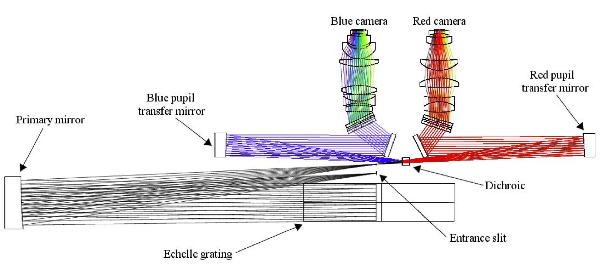
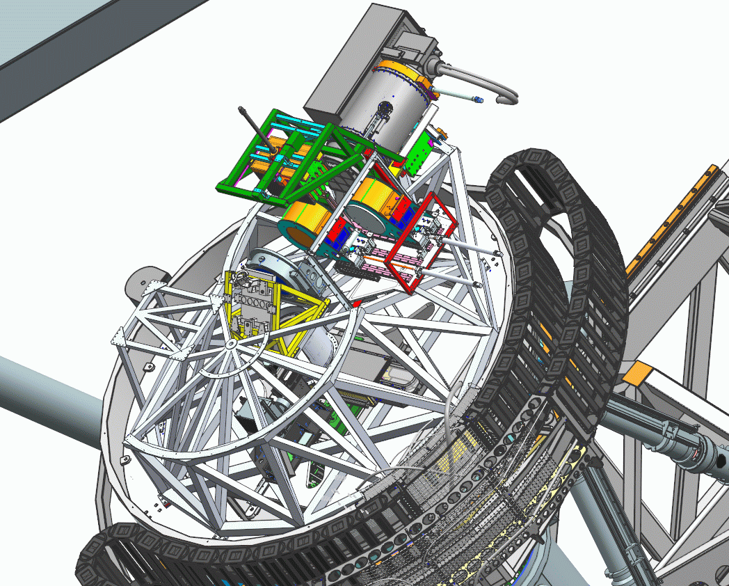
Figure 7.1: New RSS detector system with the old 3-CCD system overlaid (top). Slit position relative to the old detector for reference (bottom; old image).
binning | vertical frame size (pix) | Readout time `FAST’ mode (sec) | Readout time `SLOW’ mode (sec) |
1x1 | 6160 | 34 | 98 |
1x1 | 4096 | 24 | 65 |
… | |||
TBC |
Table 7.1: Readout speeds for FAST and SLOW readout modes for the new RSS detector. This table will be updated after full characterisation.
7.5 Gratings
RSS has a complement of six volume phase holographic (VPH) transmission gratings — see Table 7.2. All six gratings are currently installed in the magazine. The old PG0300 grating is no longer available for science. VPH gratings have the characteristic that their efficiency varies with input angle (see Fig. 7.2), and thus a single grating can cover a large wavelength range with good efficiency by changing the relative angle between the collimated beam and the grating normal. This is accomplished using a rotating stage. The RSS camera is then articulated to twice the grating angle since the VPH efficiency curve for a given grating angle typically is at a maximum at the Littrow wavelength (note that the PG0700 grating uses off-Littrow configurations). The angle of the grating also affects spectral resolution. The higher the value of the grating tilt, the higher the spectral resolving power for a given slit width.
The RSS and VPH grating simulator tools found at
http://astronomers.salt.ac.za/software/ should be used to determine the optimal grating angle and slit-width for an observation. Note also that a feature of VPH gratings is that the resolution and wavelength range of an object depends on the distance of the target from the optical axis. While this is not an issue for long-slit spectroscopy, it will affect multi-object spectroscopy (see Section 7.7.4 for more details).
All gratings are used in first order only. Second-order contamination is removed through the use of order-blocking filters (Sec 7.6).
Grating Name | Wavelength Coverage (nm) | Usable Angles (deg) | Bandpass per tilt (nm) | Resolving Power (1.25” slit) |
PG0700 | 320–900 | 3.0–7.5[1] | 400–320 | 400–1200[2] |
PG0900 | 320–900 | 12–20 | ~300 | 600–2000 |
PG1300 | 390–900 | 19–32 | ~200 | 1000–3200 |
PG1800 | 450–900 | 28.5–50 | 150–100 | 2000–5500 |
PG2300 | 380–700 | 30.5–50 | 100–80 | 2200–5500 |
PG3000 | 320–540 | 32–50 | 80–60 | 2200–5500 |
Table 7.2: RSS grating complement
Figure 7.2: VPH grating efficiency as calculated using Rigorous Coupled Wave (RCW) analysis in resolving power versus wavelength for a 1.5” slit. The contours correspond to 90%, 70%, and 50%. Wavelength coverage for a few angles is shown for each grating.
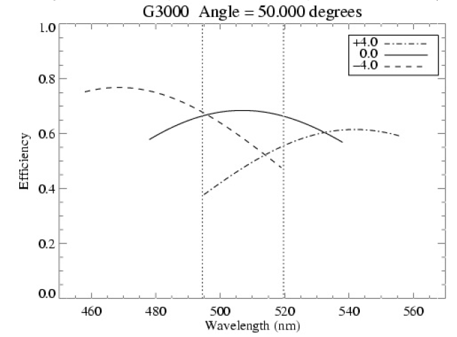
7.6 Filters
Five order-blocking filters are available for RSS spectroscopy: one clear, three UV blocking (with different lower wavelength edges), and one Blue blocking. These filters are listed in Table 7.3 and transmission curves can be found in Sec. A.6.
There are also 40 Fabry-Pérot interference filters which can also be used for narrow-band imaging; they are listed in Table 7.4. All filter transmission curves are shown in Sec. A.8.
Type | Name |
Clear | PC00000 |
UV | PC03200, PC03400, PC03850 |
Blue | PC04600 |
Table 7.3: RSS order blocking filters
Name | Centre (Å) | FWHM (Å) |
PI04340 | 4349.4 | 79.1 |
PI04400 | 4412.3 | 92.4 |
PI04465 | 4478.1 | 84.9 |
PI04530 | 4530 | 90 |
PI04600 | 4600 | 95 |
PI04670 | 4670 | 100 |
PI04740 | 4760.2 | 111.1 |
PI04820 | 4820 | 105 |
PI04895 | 4912.5 | 105 |
PI04975 | 4990.6 | 107.5 |
PI05060 | 5071.5 | 110.5 |
PI05145 | 5152.1 | 109.2 |
PI05235 | 5237 | 119.1 |
PI05325 | 5325 | 125 |
PI05420 | 5420 | 130 |
PI05520 | 5520 | 135 |
PI05620 | 5631.5 | 137 |
PI05725 | 5731.1 | 133.6 |
PI05830 | 5833.6 | 142.8 |
PI05945 | 5946.5 | 164.1 |
PI06055 | 6062.2 | 148.6 |
PI06170 | 6178.8 | 169 |
PI06290 | 6300.2 | 158.3 |
PI06410 | 6418.4 | 161.5 |
PI06530 | 6535.5 | 156 |
PI06645 | 6647.4 | 148.8 |
PI06765 | 6765 | 167.5 |
PI06885 | 6894.3 | 181.8 |
PI07005 | 7020.8 | 162.1 |
PI07130 | 7131.3 | 140.4 |
PI07260 | 7252.7 | 184.1 |
PI07390 | 7400 | 218 |
PI07535 | 7555.6 | 200.8 |
PI07685 | 7691.9 | 168.9 |
PI07840 | 7831.6 | 207.6 |
PI08005 | 7999 | 249.2 |
PI08175 | 8175.1 | 225.2 |
PI08350 | 8350 | 245 |
PI08535 | 8535 | 260 |
PI08730 | 8730 | 275 |
Table 7.4: RSS Narrow-band (Fabry-Pérot) Filters
7.7 Available instrument modes
7.7.1 Narrow-band or clear imaging
The RSS optical design is not optimised for broad-band imaging (SALTICAM is recommended instead). Narrow-band imaging may be performed with any of the 40 Fabry-Pérot interference filters listed in Table 7.4.
There was considerable fringing when using the old CCD and the red narrow-band filters when they are illuminated at discrete wavelengths. Fringing was measurable in the narrow-band filters long-ward of 750 nm: PI08350, PI08535, and PI08730 filters had obvious fringing at levels of 10–20% peak-to-trough. We expect the fringing to be less prominent using the new detector, but this still needs to be quantified.
RSS imaging can be done in frame transfer and slot modes (see Sec 7.7.6).
7.7.2 Long-slit spectroscopy (LS)
Long-slit spectroscopy is the most commonly-used mode for RSS.
A variety of slits are available to cover the range of atmospheric seeing conditions expected at the site. The choice of slit widths is driven by considerations of resolution and throughput. The instrument’s slit-mask magazine has room for ten tilted longslits. Please refer to the PIPT for the most up-to-date, full list of slitmasks available for all modes. The gratings described in Table 7.2 are available, and all order-blocking filters that are listed in Table 7.3 are also available.
Non-sidereal target spectra
Tracking at the object rates is not commissioned. However, observations of bright targets (that can be seen on the slit) whose motion is aligned along a wide slit (2” or greater) will be accepted. It is the responsibility of the PI to determine the correct position angle to keep the target in the slit and to ensure that the target is bright enough to appear in the slit view images (so that the SALT observer can push it back into the slit if it moves out). For position angle visibility documentation, see
http://astronomers.salt.ac.za/wp-content/uploads/sites/71/2014/08/SALT_PA_Visibility.pdf.
7.7.3 Slitmask IFU spectroscopy
SMI is an IFU observing mode for RSS that uses a fibre-optic retrofit with prisms mounted in a cassette. The cassette is inserted into the slit-mask magazine in the same way as the long-slit, MOS, and polarimetry masks. Both SMI-200 and SMI-300 allow integral-field spectroscopic observations using the existing suite of RSS gratings and filters.
The SMI-200 uses 200 μm fibres, corresponding to approximately 0.9 arcsec on sky, arranged in a 22.3 × 17.6 arcsec hexagonal field with a fibre-to-fibre separation of 1.08 arcsec. The SMI-300 mode uses 300 μm fibres, corresponding to approximately 1.33 arcsec on sky, and provides a larger hexagonal field of view of approximately 33.0 × 18.6 arcsec. These modes are now available for use, and more details can be found here: SMI for the SALT Call for Proposal Phase 1.
7.7.4 Multi-object spectroscopy (MOS)
RSS has multi-object spectroscopy (MOS) capability. Slit masks are laser-cut on carbon-fibre masks in Cape Town. A slit-mask magazine that has room for 30 MOS masks resides on the instrument, and all fabricated masks are stored on site.
The masks are manufactured following user specifications through a java-based RSS Slit-Mask Tool (RSMT), or a Python-based tool (PySlitmask). The latter is under development and does not have all the features available in RSMT implemented yet. These tools are downloadable from the SALT proposal tools web pages: http://astronomers.salt.ac.za/software/. Please contact salthelp if you have any difficulty installing or running the software, or if you come across any bugs.
Note that due to the way SALT operates there are restrictions in the available field orientation / Position Angles (PA) for any given RA and DEC, see http://astronomers.salt.ac.za/wp-content/uploads/sites/71/2014/08/SALT_PA_Visibility.pdf for a detailed documentation (beware the crucial distinction between `slit’ and `slot’). Slit masks will be prepared during Phase 2 proposal submission and cut after the Phase 2 submission and checks made by the Liaison SA.
No SALT pre-imaging is required for the mask preparation, provided accurate enough astrometry of the targets is available. We stress that high-quality astrometric solutions in the PI’s images are absolutely crucial for successful MOS observations, that is, 0.3” or better. Pre-imaging can be obtained with SALTICAM if required, though these require their own (time charged) Observing Blocks which have to be observed well in advance of the MOS observations. Pre-existing astrometric files are strongly preferred and the reference stars for alignment and the science slits themselves must come from the same WCS source. MOS masks use 4 – 7 5”x5” holes for reference stars and alignment is done with feedback from through-slit images.
A specific characteristic of the VPH gratings to keep in mind is that the wavelength dependence of the efficiency, as well as the simultaneous wavelength coverage for a given grating setup, depends on the input angle to the grating. In MOS, the light entering through off-axis (in the dispersion direction) slits will hit the grating at different angles. Thus, the efficiency for the off-axis objects will be different than for the on-axis objects. This will in general not be symmetric either. Figure 7.3 illustrates this, and MOS users should consult the VPH grating simulator at
http://www.sal.wisc.edu/PFIS/docs/rss-vis/ebb/pfis/observer/specsim.html
for details.

Figure 7.3: Example of the effect of blaze-angle on wavelength range and efficiency in MOS mode. Shown are the default case (on-axis) and the two extreme cases of having an object at the edges of the RSS field-of-view at ±4’ off-axis.
A new guider with two guide probes was installed in March/April 2018. It allows for the selection of fainter guide stars and eliminates rotational drift. The RMS guidance scatter is 0.”15, centred on zero, however we still recommend slits of width 1” or larger when using MOS. See Sec 7.9 for more details.
Tips and tricks
Based on the first semesters of MOS observations the three most frequent issues we have seen when executing submitted programs are:
- The tendency of PIs to underestimate the required exposure times for faint targets;
- Insufficient accuracy in the WCS of the reference stars (0.3” or better required);
- Some PIs specify too short slits (that is, <10”) which will make sky-subtraction very difficult.
A set of instructions for preparation of MOS Phase 2 material, including e.g. proper selection of reference stars, can be found from the MOS specific Phase 2 FAQ page at
http://astronomers.salt.ac.za/proposals/mos/.
7.7.5 Polarimetry imaging / spectropolarimetry
Polarimetry modes using RSS are (not all available yet):
- Point-source long-slit linear spectropolarimetry with any grating and setting [available]
- Point-source long-slit circular and all-stokes spectropolarimetry [available]
- Diffuse long-slit spectropolarimetry (with spatial information) [available]
- Multi-object (MOS) grating spectropolarimetry [not available]
- Imaging spectropolarimetry (using beamsplitter cross-dispersion in imaging mode) [not available]
We ask that those interested in any unavailable modes should contact salthelp@salt.ac.za with their preferences by the same Phase 1 deadline.
We also encourage users to read to the Polarimetry Observer’s Guide as this document includes a description and capabilities of the various modes. This document more importantly instructs users on how to construct a proposal and use the PIPT to define polarimetric observations.
We note here that revised calibrations for linear polarization, taken with the PG0900 grating, will be released this semester. These calibrations aim to remove the dependence on track position which can mainly be seen in the PA as a "ripple" in wavelength, stretching over several hundred Angstroms. A new version of polSALT will accompany this release.
Polarimetry users wanting to use the PG0700 grating should note that only data taken with grating angles of 3, 4.6 and 7.5 degrees can currently be reduced with the polSALT software. Reduction of data taken with any other grating angles will not be supported at present. PIs wanting to use other angles should discuss with AstroOps by sending an email to salthelp@salt.ac.za by the same phase 1 deadline.
Polarimetric optics
The RSS polarimetric optics employs a “wide field” design, in which a polarizing beamsplitter in the collimated beam takes the central half of the field and splits it into two separate orthogonally polarized fields, the “ordinary” (O) and “extraordinary” (E) beams. One (or two) waveplates can be inserted into the beam, right after the field lens in the collimator, to modulate the polarization state with time. The difference between the intensities of the O and E images as a function of time as the waveplates are rotated yields the polarization. For the polarimetric modes, only the central 4-arcminute portion of the focal plane is used (accomplished using a short slit for spectroscopy or a special mask blocking the upper and lower quarter of the field of view for imaging), see Fig. 7.4.

Figure 7.4: FoV for long-slit spectropolarimetry
Waveplate patterns
The waveplate modulators are used in five modes with specific, predefined patterns: Linear, Linear-Hi, Circular, Circular-Hi, and All Stokes. For ease of operation, the waveplates are in the same order in all modes, half wave first. Table 7.6 gives the wave-plate angle exposure progression pattern for each mode. The angle shown is that between the waveplate optical axis and the beam splitter polarization axis, which is perpendicular to the dispersion direction. A dash (–) means that the waveplate is not inserted.
Linear | Linear-Hi | Circular | Circular-Hi | All Stokes | |||||
½ wave | ¼ wave | ½ wave | ¼ wave | ½ wave | ¼ wave | ½ wave | ¼ wave | ½ wave | ¼ wave |
0 | – | 0 | – | 0 | 45 | 0 | 45 | 0 | 0 |
45 | – | 45 | – | 0 | -45 | 0 | -45 | 45 | 0 |
22.5 | – | 22.5 | – | 22.5 | -45 | 22.5 | 0 | ||
67.5 | – | 67.5 | – | 22.5 | 45 | 67.5 | 0 | ||
– | 11.25 | – | 45 | 45 | 0 | 45 | |||
– | 56.25 | – | 45 | -45 | 0 | -45 | |||
– | 33.75 | – | 67.5 | -45 | |||||
78.75 | – | 67.5 | 45 |
Table 7.6: RSS Polarimetry waveplate patterns
PIs will need to select a waveplate pattern depending on the nature of the observation:
- Linear: Faint object linear polarization (minimises exposures).
- Linear-Hi: High-precision linear polarization; redundant information gives systematic error estimate.
- Circular: Faint object with substantial ellipticity (circular/linear ratio).
- Circular-Hi: Object with low ellipticity; redundant information to estimate linear-to-circular contamination.
- All-stokes: Linear and circular.
The full pattern must be completed to yield the Stokes parameters.
We give the following advice when planning Phase 1 or defining Phase 2:
- In the simulator, select the flag “use polarimetry”, and in the PIPT select the polarimetric mode from the Mode dropdown menu: both settings offer the following choices.
- Slit Type: only “Longslit” is currently available.
- Slit Width: use the PIPT, not the simulator selection, for the currently available longslits.
- Gratings: all stations and angles are available for gratings. Imaging polarimetry (slit/grating not set) is not yet fully commissioned.
- Always request guided observations (poor guidance can introduce spectropolarimetric features).
For an estimation of expected S/N of linear spectropolarimetric features use the simulator SN prediction (p = 1/SN). For baseline (“instrumental") linear polarization repeatability, assume 0.1–0.2%. This may improve during the semester as more calibration data is obtained, and the analysis software improves. It is very possible that, especially with the VPH gratings, there is a track position dependence of the linear polarization baseline at that level, which is under investigation. If this is of concern, plan on doing everything twice to assess these sort of systematic errors.
We again encourage users to read to the Polarimetry Observer’s Guide as this document includes a description and capabilities of the various modes. This document more importantly instructs users on how to construct a proposal and use the PIPT to define polarimetric observations. The analysis software is available at https://github.com/saltastro/polsalt. PIs are encouraged to contact salthelp@salt.ac.za should they need any assistance.
7.7.6 High-speed imaging and spectroscopy
RSS imaging can be done in high-speed mode, that is, in frame transfer and slot modes. However, these modes have not yet been finalised for the new detector, so details such as the minimum exposure times are not yet known for sure. Table 7.7 shows our estimates from preliminary testing in the lab at IUCAA, for a 200 pixel ‘slot’. Note that these are significantly slower than with the old detector.
Frame Transfer and slotmode spectroscopy are currently available with a 1.5” or 2.0” slit, but please contact the SALT team should you require a different slit width.
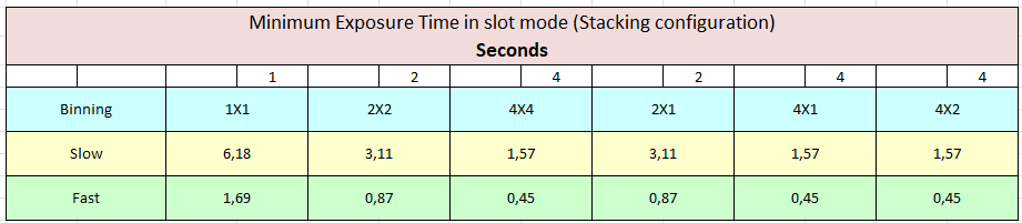
Table 7.7: Minimum exposure times for Frame Transfer and Slot mode for RSS (new detector).
7.8 Sensitivity
All RSS sensitivity calculations for planning observations should be done with the latest version of the RSS Simulator. PIs are warned that the RSS throughput below 400 nm is not nearly as good as expected originally. See Section 4.3 and Figure 4.3. for more information. All current information on both the telescope and instrument throughput based on recent measurements is incorporated into the RSS Simulator.
However, we have noticed through experience that PIs often underestimate the required exposure times, especially with fainter targets: Please be conservative when selecting the conditions for the simulation, and remember the IQ and seeing definitions (Secs 4.1 and 3.6.2, respectively) and that seeing and image quality has a large effect on the S/N of targets fainter than sky brightness. In addition, be sure you understand different definitions of S/N (that is, per pixel or per resolution element) and what these mean for your science.
We note that in the past there was straylight reaching the RSS detectors decreasing the S/N of faint observations due to elevated background levels. This issue has long since been fixed and during 2015 we determined that straylight levels are far below the normal night sky levels on RSS. Tests for straylight are done regularly. The Sutherland night sky levels were determined to be dark, similar to the Paranal night sky.
As a guideline, approximate magnitude limits at a mid-range wavelength for each grating are tabulated in Table 7.8. The numbers are applicable to long-slit and MOS observations close to the centre of the FoV (the sensitivity in MOS decreases with distance from the centre). The magnitude limits have been estimated based on experience, taking into account the degraded SAC. They have yet to be quantitatively determined for the new detector.
Grating | Central λ (nm) | Resolution (λ/δλ) | Mag Limit (V) |
PG0700 | 610 | 800 | 20.5 |
PG0900 | 605 | 1065 | 20.5 |
PG1300 | 665 | 1800 | 20.0 |
PG1800 | 677 | 2890 | 19.5 |
PG2300 | 566 | 3220 | 19.5 |
PG3000 | 434 | 3215 | 19.0 |
Table 7.8: Guideline RSS sensitivities – yet to be precisely determined for the new detector. The RSS Simulator tool should be used for more detailed calculations.
7.9 Guiding
The RSS auto-guider is routinely used for all RSS observations. It was upgraded in March 2018. It has two cameras available, one for each half of the field of view, and is much more sensitive than the previous guider, easily reaching guide stars at V ~ 18 mag. Guiding capability was significantly improved, particularly for MOS where the available field for selecting a guide star may be much more restricted. The system also corrects for any residual rotational drift and provides auto-focus capability. The new guide probes can position the field to approximately 0.1” RMS.
7.10 Blind offsets, dithering and nodding
Point sources fainter than approximately 19 mag in dark time, and 17 mag in bright time may not be visible to be put on the slit in several second long acquisition images. The exact limit depends greatly on seeing at the time of observation as well as on the diffuseness of the target – the number above relates to point sources in 1.5” to 1.8” seeing. To put fainter targets on the slit, other methods are needed.
Our current positional accuracy and repeatability is ~0.1” RMS while guiding, measured by performing offsets of sizes varying from 0.5” to 30” and returning to the original position. If this accuracy is sufficient for blind offsetting, e.g. for targeting more diffuse sources, and/or when using wide slits, blind offsetting is operationally feasible and may be requested in an ad hoc manner by discussing it with the liaison astronomer.
In most cases, however, we recommend providing a brighter alignment object and a PA that will ensure placement of the fainter object in the slit. The PA positioning accuracy is at least 0.5 deg, probably better, so finding a star of V=15–17 mag at <60” distance would ensure the positioning of the slit with <0.5” accuracy. It is safer to use slit widths of 1.5” or more, and to use alignment stars as close as possible (<60”) to the target.
All of the comments and caveats about SALTICAM dithering that are discussed in Sec. 6.8 apply to RSS as well. The accuracy of the dithering is limited currently to 0.5” RMS. For some purposes, this is perfectly fine. For others (e.g. dithering blindly between different slit positions), it may not be. However, since in most cases an object will be visible on the slit-viewer, the observer just would re-check alignment before re-starting exposures (60 sec overhead is defined for dithering along the slit, which includes the move and tweak of position if required).
Nod-and-shuffle mode is not currently offered.
7.11 Calibrations
Please note that this section has not been updated for the new detector, and is merely a copy from the 2026-1 call for proposals. Details will be relayed to users after calibrations are taken with the new system. We do not expect any significant changes in wavelength related calibrations, as we are not touching optics nor changing the width or plate scale of the CCD.
Please refer to Sec. 5 for a general description of SALT calibrations. All calibrations should be requested by the relevant check-boxes in the Phase 2 PIPT. The PIPT tool to build observing blocks includes all overheads. For a quick overview of relevant overheads see Sec. 9.
7.11.1 Features of RSS calibrations
The RSS calibration plan (see below) is based on the SALT telescope specifications and on current experience. We would like to point out the following:
- SALT is a telescope with a variable pupil so the illuminating beam changes continuously during the observations. This makes it impossible to perform absolute flux calibration even using spectrophotometric or photometric standards.
- Our current experience shows that biases are only useful for RSS Faint/Slow mode. Bias for this mode are now taken nightly as part of the default calibration process (2x2, 4x2 and 4x4 binning). A report discussing these biases is available at:
https://sciencewiki.salt.ac.za/index.php/A._Schroeder_RSS_Bias_analysis
- Imaging Mode: Everything described in Sec. 6.10.1 about SALTICAM flat-fielding also applies to RSS imaging.
- Long-slit Mode:
- At least one in-focus SALTICAM slitview (acquisition) image will be provided.
- Unless reference spectra (arcs) are obtained immediately before, after, or between science observations, wavelength calibration solutions may shift up to 10–14 unbinned pixels during a 900s exposure: 0.5–0.7 nm for grating PG0900 and 0.1–0.2 nm for PG3000, see
http://wiki.salt.ac.za/images_wiki.salt.ac.za/3/31/RSS_stability.pdf
- For reference spectra we guarantee that the RMS uncertainty of 2D wavelength solutions will be at most ½ of an unbinned pixel for most of the spectral setups: 0.025 nm for PG0900 and 0.008 nm for PG3000.
- Due to flexure within the spectrograph, spectra can have trends in their wavelength solutions of up to 1 unbinned pixel in a 900s exposure.
- Each slit has some variations in throughput along the slit due to roughness in the slit edges. These variations are up to 10% row-to-row and can shift significantly due to spectrograph flexure and lack of mechanical repeatability. To correct for this effect, spectral flats must be obtained immediately before or (preferably) after science frames.
- Spectral pixel-to-pixel variations are also corrected using spectral flats. These corrections can decrease the background RMS for data up to 5%. At the same time “lazy pixels” can be corrected for up to 95% of their difference in sensitivity.
- The map of spectral pixel-to-pixel variations is roughly constant with a maximum of 10–20% variation over a week’s time.
- Fringing correction: Beyond approximately 7500 Å there is significant fringing present on the spectral frames, and spectral flats (calibration screen flat fields) taken together with the science frames are essential for all target types to reduce for this effect. In addition, for both sky and fringing removal for fainter and/or extended targets at these reddest settings it is also helpful to dither along the slit between the (two or more) science frames. The dither step must be larger than the extent of the target. A report on the findings and suggestions is available at https://sciencewiki.salt.ac.za/images_sciencewiki.salt.ac.za/1/12/SALT_RSS_fringing.pdf
- MOS mode: MOS calibrations are equivalent to long-slit calibrations. Arcs and flats will be taken through the PI-specified mask. However, the spectrophotometric standard will be taken with a 4” long-slit using otherwise the same RSS configuration, hence directly applicable only to those slitlets that happen to lie on-axis.
- Fabry-Pérot mode: Unavailable.
7.11.2 Current RSS calibration plan
The calibration plan (see Sec. 5 for definitions) for RSS for the upcoming semester is:
- No DC calibrations will be done
- No LC calibrations will be done
- UCC calibrations will be done by PI request and the PI will be charged accordingly. These include:
- Long-slit mode:
- Observations of any reference arc spectra before / in between / after science observations. For each reference arc spectrum the PI will be charged at least 120 sec because of the time it takes to configure the calibration system and the integration time required to obtain a good arc spectrum (sometimes 60 sec). For increased efficiency, we recommend the arc observation to occur after the science if only one set is needed. Arcs are highly recommended to be taken for every Observing Block.
- Observations of 5 spectral flats before / in between / after science observations. For each set of 5 spectral flats the PI will be charged approximately 120 sec, which includes the setup, integrations and readouts. We recommend spectral flats be taken after science for efficiency. For clarity, we ask that the PI clearly mentions in both Phase 1 and Phase 2 whether or not flats are needed.
- UNC calibrations can be done by PI request:
- Long-slit mode:
- Observations of one spectrophotometric standard star (1 exposure) per detector and spectrograph setup. These observations will be taken with the widest available long-slit (normally 4”). The star will be placed in the middle of the slit. These data will be acquired during the next available twilight. Note that arcs and flats are not normally taken for spectrophotometric standards (the sets coming with the science exposures should be sufficient). For clarity, we ask that the PI clearly mentions in both Phase 1 and Phase 2 whether or not spectrophotometric standards are needed for the science. Finally, note that if a specific standard star needs to be observed, or the PI wants arcs/flats with the star, these are charged.
- Observations of one Lick standard star (1 exposure) per detector and spectrograph setup. The star will be placed in the middle of the slit. These data will be acquired during the next available twilight. See comments above. If the PI requires a specific spectral type, this must be clearly indicated.
- 5 spectral (lamp) flats per detector and spectrograph setup taken during the day or twilight. These can be requested instead of the charged UCC flats taken during the night time after the science frames. However, we do NOT recommend the use of these UNC flats except for pixel-to-pixel corrections. Because the pixel-to-pixel variation is stable, we will take such flats only once per semester for a given setup. The illumination and, especially, the variations due to slit non-uniformity ARE NOT repeatable.
- 3–5 twilight spectral flats followed by an arc taken with the same slit width and setup as the science data will be taken upon request during the next available twilight. However, since these observations are very time-consuming the request needs prior approval from the liaison astronomer.
- Imaging mode:
- 5 calibration screen flats per detector and spectrograph setup taken during twilight or day.
- 11 biases per detector setup.
8. HRS
8.1 Current status
HRS is available and routinely being used in all of its modes (LR, MR, HR and HS) but with one default detector configuration: 1x1 binning, single amplifier, slow readout. See Sec. 8.4.1 for a brief discussion on mode availability.
8.2 Characteristics and performance
The SALT HRS is a dual-beam (blue: 370 – 555 nm, and red: 555 – 890 nm) fibre-fed, white-pupil, échelle spectrograph, employing VPH gratings as cross dispersers. The cameras are all-refractive. The concept is for SALT HRS to be an efficient single-object spectrograph using pairs of large (350 μm to 500 μm; 1.6 -- 2.2 arcsec) diameter optical fibres, one for the source (object) and one for the background (sky). Some of these feed image slicers before injection into the spectrograph, which deliver resolving powers of R ~14000 (unsliced 500 μm fibres), ~40000 (sliced 500 μm fibres), and ~65000 (sliced 350 μm fibres). A single 2k x 4k CCD is sufficient to capture all the blue orders, while a 4k x 4k detector, using a fringe-suppressing deep-depletion CCD, is used for the red camera. Complete free spectral ranges are covered by both the blue and red arms. The spatial resolution is ~0.3 arcseconds. The accuracy of HRS radial velocities is better than 200 m/s for the low resolution mode and 150 m/s for the medium and high resolution modes.
8.3 Detector
The blue arm has an e2v CCD 44-82 blue detector which is thinned and back illuminated. It has a broadband anti-reflective coating applied. The pixel format is 2048 x 4096 (15μm pixels). The red arm has an e2v CCD 231-84 with 4096 x 4096 pixels (15μm pixels). This chip is manufactured from deep depletion silicon and has the Extra Red Plus fringe suppression option. The fringe suppression process attenuates the internal interference fringes seen at long wavelengths (>800 nm) on thinned, backside illuminated CCDs.
The quantum efficiency of the red CCD is 93.1% at 650 nm and decreases to 58.4% at 900 nm. For the blue CCD it is 90% at >500 nm and falls to ~74% at 400 nm.
8.4 Readout modes
HRS supports a variety of detector read-out modes, with users able to tailor read-out speed, binning and the number of read-out amplifiers to suit their needs. Modes and read-out speeds are summarised in Tables 8.1 and 8.2 below.
1000kHz and 400kHz read-out speeds are supported on both detectors. The former offers a shorter read-out time at the expense of marginally higher read-out noise. 1000kHz should offer acceptable read noise performance in many circumstances (the values in Table 8.1 are averaged over all two/four read-out amplifiers for blue/red CCDs, respectively).
CCD binning options are 1x1, 2x2, 3x3, 8x8 and 3x1 (that is, binning in the spatial direction only). 1x1 binning is the standard binning mode, since binning will degrade spectral resolution in all but the low resolution mode (where a resolution element is multiple pixels in width). Despite no binning in the spectral direction, the 3x1 binning mode will still cause some resolution loss in all but the low-resolution mode, since it will smear the effect of line tilt across the order. The advantages of binning are reduced read-out times and reduced read-out noise, since fewer ‘pixels’ are read-out.
It is possible to read-out the detectors using single or multiple read-out amplifiers. For the 2k x 4k blue CCD, the options are one or two amplifiers. In the case of the larger 4k x 4k red CCD, the options are one or four read-out ports. Read-out speed scales with the number of amplifiers (so four amplifier read-out is four times faster than a single amplifier at the same speed and binning). Note that when using multiple read-out amplifiers, each area of the chip will have a different bias level and overscan region, which must be dealt with in the data reduction process.
Note that the HRS CCDs are read out in series rather than in parallel, as parallel read-out can cause a small cross-talk signal between the detectors. The blue CCD is therefore read out before the read-out of the red CCD commences. Read-out times reflect the sum of the two read-outs. For example, running three back-to-back iterations of 10s exposures using the standard detector settings would take 3 x (10s + 23s + 37s) = 210s.
1000kHz | 400kHz | |
Red | 4.7e- RMS | 3.6e- RMS |
Blue | 5.8e- RMS | 4.2e- RMS |
Table 8.1: HRS red and blue detector read-out noise with different read-out speeds.
Red | 400kHz | 1000kHz | ||
Binning | Single | Quadruple | Single | Quadruple |
1x1 | 37s | 10s | 19s | 5s |
2x2 | 11s | 3s | 6s | 2s |
3x3 | 6s | <2s | 4s | <1s |
3x1 | 13s | 4s | 7s | 2s |
Blue | 400kHz | 1000kHz | ||
Binning | Single | Double | Single | Double |
1x1 | 23s | 12s | 10s | 5s |
2x2 | 8s | 4s | 5s | 3s |
3x3 | 5s | 3s | 3s | 2s |
3x1 | 8s | 5s | 4s | 2s |
Table 8.2: HRS red (top) and blue (bottom) detector read-out times (in seconds) with different binning and read-out amplifier configurations. The default (=standard) readout mode is highlighted.
8.4.1 Caveats and recommended readout modes
Users are strongly advised, in almost all cases, to use the standard detector configuration as indicated in Table 8.2 for HRS proposals. Although it is the slowest option, the data quality will be of the highest achievable standard, with the simplest possible data reduction requirements. SALT will provide the calibration files (weekly CalSys arcs and flats for all resolution modes; daily HS internal ThAr mode arcs; daily bias frames, see Sec. 8.9.2). This read-out mode is also currently the only one which is fully supported by the data reduction pipeline. Users using other modes will only receive the raw data and will have to process the data themselves.
Alternatively, in extreme and specialist circumstances, users may request a configuration other than this default read-out option. In order to accommodate such a request, additional calibration frames in the requested new custom read-out mode will have to be created in addition to the standard ones. Clearly it is unfeasible to offer every possible read-out configuration (there are 20 possible read-out mode combinations per detector), as the calibration requirements would be vast. It will be thus the responsibility of the PI to provide a detailed and valid technical motivation.
As an example, a hypothetical proposal with one target, one visit and 2x1800s exposures on a bright star in low-resolution mode, might prefer to use multiple amplifiers, 1000 kHz read-out speed and 3x3 binning. SALT would not support such a request merely to save the proposer 117s of read-out time at 3600s of observing time.
On the other hand, a hypothetical proposal with 40 visits of 3x2s exposures for, e.g., an exoplanet monitoring program could make a reasonable argument to use a 1000 kHz read-out configuration. Since overheads make up the bulk of the time in this case (a reduction from 7200s to 3480s overheads for 240s observing time), AstroOps may consider granting such a request at their discretion. Another good example is a scientific requirement for high time-resolution observations requiring low read-out overheads.
Although an 8x8 binning option is available for HRS, the various gains in 8x8 mode for each CCD amplifier have not been empirically determined. For this reason, in addition to those mentioned above, 8x8 binning should be avoided until proper detector characterisation has been obtained.
8.5 Operational modes
SALT HRS offers four different operational modes, which vary in spectral resolution at the expense of instrument throughput. Table 8.3 summarises the four modes along with their characteristics and options.
Parameter | Low Resolution Mode | Medium Resolution Mode | High Resolution Mode | High Stability Mode |
Fibre Diameter (μm) | 500 | 500 | 350 | 350 |
Fibre Diameter (arcsec) | 2.23 | 2.23 | 1.56 | 1.56 |
Slit width (arcsecs) | 1.673 | 0.710 | 0.355 | 0.355 |
Image Slicers | No | 3 slices | 3 slices | 3 slices |
Blue arm resolution | 15000 | 43000 | 65000 | 65000 |
Red arm resolution | 14000 | 40000 | 74000 | 65000 |
Blue arm transmission (total %) at 460 nm* | 12 | 7 | 7 | 4 |
Red arm transmission (total %) at 625 nm* | 19 | 11 | 12 | 6 |
Fibre mode scrambling | No | No | No | Yes, permanent |
Nod and shuffle | Optional | No | No | No |
Iodine cell | No | No | No | Optional** |
Simultaneous ThAr** | No | No | No | Optional** |
Total photon count*** | Yes | Yes | Yes | Yes |
Table 8.3: Summary of HRS mode characteristics and efficiency predictions.
* These efficiency values represent the as-measured ‘end-to-end’ throughput for the spectrograph as a whole, including the optical fibre feed.
** Note that the Iodine cell and simultaneous ThAr feed cannot be used simultaneously.
*** From an exposure metre (unless using the optional internal ThAr lamp in simultaneous use in the high stability mode).
8.5.1 Low resolution mode (LR)
This is the lowest resolving-power R = 14000 configuration. The configuration offers the same fibre input diameter as the R = 40000 (MR) mode (that is, 500 μm) but with the benefit of a 1.4 × higher throughput because the fibre output is not image-sliced (hence the coarser resolution).
Examples where the lowest resolving power may be tolerable and where the improved background sampling might be beneficial include spectroscopy of diffuse interstellar bands against lines of sight to distant stars or quasars and molecular band analyses of stars in Local Group galaxies.
8.5.2 Medium resolution mode (MR)
The R = 40000 mode is the most commonly used SALT HRS mode. It has adequately high resolving power for many projects but with a larger fibre diameter and higher throughput than the R = 65000 (HR) mode. Studies of objects whose intrinsic line widths are broader than two resolution elements of the R = 65000 mode, such as rotating stars (e.g. most O and B stars), stars in which the Balmer line strength measurements are the principal aims, and studies of molecular bands at medium resolution are likely to benefit from the resolving power versus throughput trade-off available in this mode.
8.5.3. High resolution mode (HR)
The R = 65000 mode is useful only for those projects for which the lower throughput compared to the R = 40000 mode is more than offset by the greater resolving power. Such observing projects include studies of line profiles in investigations of stellar atmosphere dynamics, resolving closely spaced lines, or the study of absorbing structures in the interstellar or intergalactic medium at the highest velocity resolution. Studies that benefit from fine sampling of the stellar line profiles, such as the most precise radial velocity work, will also utilise this resolving power. Recall, however, that the wavelength stability of the instrument as a whole will be much higher than in traditional non-vacuum spectrographs, and astronomers may find they can achieve adequate velocity accuracy even at R = 40000 because of the improved systematics compared to other spectrographs.
8.5.4 High stability mode (HS)
The high stability mode is optimised for precision radial velocity measurements and is implemented at R = 65000, because of the importance of adequately sampling the line profiles in order to achieve sub-resolution-element accuracy (an error of 5 ms-1 corresponds to 10-3 of a resolution element). The light path in this mode includes a permanent ‘double scrambler’ to improve the radial scrambling of the optical fibres and reduce the spectral shifts due to the star moving on the input face of the fibre. In this mode it is also possible to place an Iodine cell into the beam (both channels) to provide a superimposed set of wavelength reference lines in the 500 – 620 nm range, or to illuminate the second (sky) fibre with an internal ThAr calibration source to obtain a simultaneous wavelength calibration. The efficiency of this mode is therefore expected to be ~50 – 70% of the normal high resolution mode and would normally only be used where this level of wavelength stability is essential. It should be noted that a new fully characterised Iodine cell has been obtained and it is available for regular operations (but please contact AstroOps for more information if you are interested in this mode). It should also be noted that the simultaneous ThAr and Iodine cells may not be used together. A laser frequency comb for high precision wavelength calibration is under development.
8.5.5 HRS Resolution Measurements
The study of FWHM and R values for LR, MR and HR modes of HRS were done using many lines (about 600) from reference spectra. The studied lines were distributed over the whole spectral region. This study shows that the measured R is slightly better for LR mode (16200 – 15800 for the Blue channel and 16500 for the Red; see Table 8.3 for the comparison), but starts to be slightly worse for MR (36500 – 38500 for the Blue and 39000 for the Red channel) and is much worse for HR mode (44000 – 46000 for the Blue and 47500 – 45500 for the Red channel). The only explanation of this effect is that the current version of the HRS MIDAS pipeline does not take the tilted nature of lines in HRS spectra into account (read this report for more details).
The most important conclusion is that in the current situation users who observe with HRS HR mode lose slightly in sensitivity compared to MR, but have an increase in resolution of only ~20% compared to the declared ~85%, because of the current version of the HRS pipeline (HRS Pipeline — SALT for Astronomers). Users do not lose this information, but the HRS pipeline is not yet able to extract the information for them.
8.6 Spectral format
Figures 8.1 and 8.2 illustrate the echellogram maps of the red and blue arm spectra as they appear on their 4k x 4k and 4k x 2k detectors respectively. The cross-over wavelength between the two arms is at 555 nm, with the blue arm covering 370 – 555 nm and the red detector covering 555 – 890 nm.
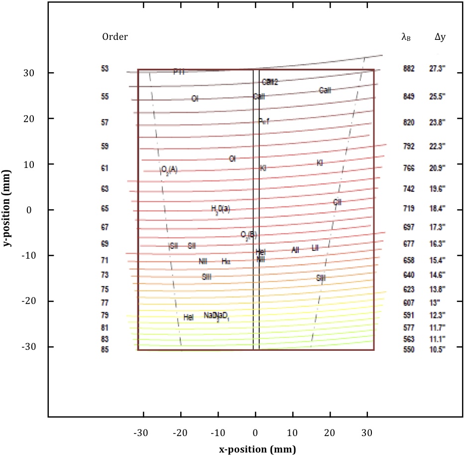
Figure 8.1: Wavelength coverage for the red arm of SALT HRS. Key spectral features are noted on each image, as are order numbers and the blaze wavelengths λB.
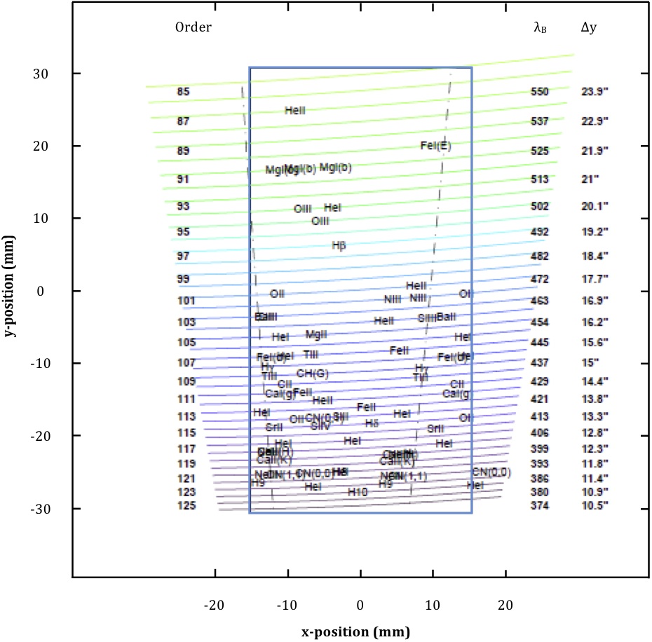
Figure 8.2: Wavelength coverage for the blue arm of SALT HRS. Key spectral features are noted on each image, as are order numbers and the blaze wavelengths λB.
8.7 Stability of radial velocities (RVs)
The standard HRS data pipeline (MIDAS, see HRS Pipeline — SALT for Astronomers for more details) makes use of the daily and weekly obtained calibration files (see Sec. 8.9.2). A Velocity Standard (RVST) star, observed in all HRS modes, is similarly reduced, and its velocity is measured and compared with the velocity from the RV catalogue. As shown in this HRS Stability report, the accuracy of HRS radial velocities is better than 200 m/s for LR mode and 150 m/s for MR and HR modes for this scheme of library calibrations. As an example, our study for the MR mode is shown in Fig. 8.3, where all library calibrations were done during the same night.
Figure 8.3: The comparison of measured velocities with their catalogue values for RV standards obtained with the MR mode over a two month period. The difference between the calculated velocity and velocity from the catalogue for each spectrum is shown with black dots. 1-sigma errors are shown with bars. The calculated average value for the total sample is shown with the horizontal long dash line (blue colour for the blue arm, red for the red arm and black for blue+red arms) and 1-sigma errors for the total sample are shown with green long dash lines.
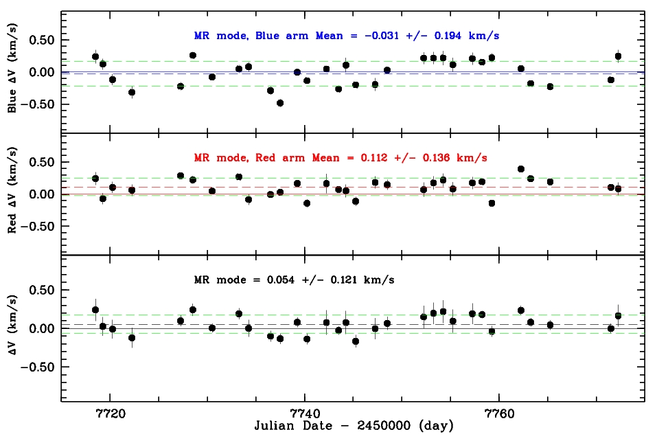
We also studied the stability of the RV determination versus the difference in days between the date of observation and date of other library calibrations. An example from such a study is shown in Fig. 8.4. The top panel shows the difference between the calculated velocity and the catalogue velocity versus the difference in days between the date of observation of the RVST and the date of other library calibrations. The weighted averages for many measured stars are shown together with the calculated error.
Figure 8.4 also shows that for the MR mode both blue and red arm data do not show any obvious systematics if calibrations were done not on the same day but within 5 – 7 days of the observation. It is thus easy to get an accuracy of less than 150 m/s using both arms’ data or only the red arm.

Figure 8.4: The comparison of measured velocities with their catalogue values for RV standards obtained with the HRS MR mode depending on the time (in days) between calibrations and science observations. The calculated average value for the total sample, as described in Fig. 8.3, is shown with horizontal lines. In this case it is coincident with Delta Days = 0. The weighted average of the calculated difference between measured velocity and velocity from the catalogue are shown for each date.
8.8 Performance prediction
Figures 8.5 and 8.6 show the anticipated signal-to-noise ratio of SALT HRS as a function of stellar visual magnitude (mv). Note the difference in performance of the four instrument modes due to variance in throughput. These values are currently based on predicted instrument efficiencies (see below for on-sky comparisons). Users may simulate HRS observations using the simulator tool available at Software — SALT for Astronomers. PIs are strongly encouraged to only split up exposures for faint objects into smaller ones if they are studying short-term variability. Splitting up exposures will result in more noise than in undivided exposures and cosmic rays can be cleaned effectively in the undivided exposures.
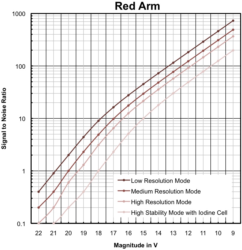
Figure 8.5: The expected signal-to-noise ratio (S/N) of SALT HRS as a function of stellar visual magnitude (mv) using the red instrument arm and a variety of operational modes. The calculations are for a wavelength of 725 nm and the low (R~14000), medium (R~40000) and high (R~65000) spectral resolving powers. A blackbody object with surface temperature of 5500K, 2 arcsec FWHM seeing at the fibre input, exposure time of 1800 sec and a telescope airmass of 1.3 are assumed. The sky brightness is calculated assuming the moon to be at first quarter. The S/N is for each extracted half-resolution element at the échelle blaze peak.
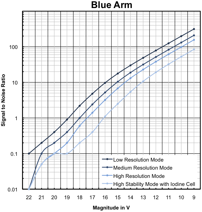
Figure 8.6: The expected signal-to-noise ratio (S/N) of SALT HRS as a function of stellar visual magnitude (mv) using the blue instrument arm and a variety of operational modes. The calculations are for a wavelength of 460 nm and the low (R~14000), medium (R~40000) and high (R~65000) spectral resolving powers. A blackbody object with surface temperature of 5500K, 2 arcsec FWHM seeing at the fibre input, exposure time of 1800 sec and a telescope airmass of 1.3 are assumed. The sky brightness is calculated assuming the moon to be at first quarter. The S/N is for each extracted half-resolution element at the échelle blaze peak.
8.8.1 On-sky measurements
We have verified that a bright object (V = 6 – 10 mag) throughput is consistent with the simulator tool predictions. Due to the on-sky size of the fibres, it is possible to observe faint targets with HRS but there are several indications that for the faintest targets (V > 16), the simulator overestimates the signal-to-noise ratio. Thus PIs are urged to be conservative in planning fainter target HRS observations, and should consider carefully whether to observe targets fainter than V = 18 even with the LR mode.
8.9 HRS calibrations
Please refer to Sec. 5 for a general description of SALT calibrations. All calibrations should be requested by the relevant check-boxes in the Phase 2 PIPT. The PIPT tool observing blocks includes all overheads. For a quick overview of relevant overheads see Sec. 9. Please note that the MIDAS pipeline is run with the appropriate calibration data.
8.9.1 Features of HRS calibrations
Our current HRS calibrations plan (see below) is based on the specifications of the SALT telescope and our current experience. Please note that users who use the outputs from the MIDAS pipeline will not require these calibration files. We would like to highlight the following:
- The standard readout mode (unbinned, single-amplifier, slow readout) comes with a default (uncharged) set of 11 bias frames taken daily. Other readout configurations are not supported, and the PI is requested to justify such a configuration and the required calibration plan will be charged.
- The weekly observed flat fields are used mostly for order definition and considered sufficient. Additional flat fields with the Iodine cell in the beam for the HS mode may be requested but, given the stability of the instrument, these are not expected to change except in the unlikely event of detaching and reattaching the fibres or opening the vacuum tank. In such a case a full set of calibration files will be taken immediately.
- Wavelength calibration for the LR, MR and HR modes is undertaken using the SALT Calibration System (CalSys) and consists of a set of ThAr hollow-cathode lamp spectra obtained through both object and sky fibres. These (uncharged) calibrations are taken during bad weather or in the daytime, weekly for these modes. In the case of the HS mode, the instrument’s own internal ThAr arc lamp is used for daily monitoring of the RV stability of HRS and arcs are thus available to the user. Results of monitoring HRS HS arcs indicate a total variation of +/– 0.4 pixels since the last time the vacuum tank was opened in August 2024, and <1/10th of this over timescales of days. For intra-night arc drifts, once the systematic trends are removed, the rms fluctuations are ~0.005 pixels (8 m/sec). For the other modes (LR, MR & HR), stability is expected to be <0.1 pixel.
- RV standard stars are normally observed with the LR, MR, HR and HS modes during twilight or during gaps in the observing queue (at no cost). These may be requested (as indeed can other standards or calibrators) at other times during the night, but will be charged for as UCC (Sec. 8.9.2). Note that due to availability or weather conditions, twilight standards may not always be observed on the same night as science data. A request for specific calibration stars should be made as for any other science target.
- Spectrophotometric standard stars are normally observed with LR, MR and HR modes in the same way as for RV standard stars, though only monthly. We will consider adding observations for the HS mode, depending on user requests.
SALT HRS is equipped with an exposure metre, which is available for use in all four operational modes (with the exception of the high stability mode when the simultaneous internal ThAr lamp is in use). Time-indexed photon counting data should therefore be available, as well as flux-weighted mid-points for the exposures.
8.9.2 Current HRS calibrations plan
The calibration plan (see Sec. 5 for definitions) for HRS for the upcoming semester is:
- DC: 11 bias frames for all modes plus two spectra of internal ThAr arc lamps for HS mode only are taken nightly as default calibrations
- LC will be taken with a period of 5 – 7 days to calibrate the standard HRS pipeline:
- Three spectral flats using the quartz-tungsten-halogen (QTH) lamps for three modes: LR, MR, HR
- Nine spectral flats using the quartz-tungsten-halogen (QTH) lamps for the HS mode
- One ThAr arc for modes: LR, MR and HR
- One Velocity Standard (RVST) star for all four modes: LR, MR, HR and HS (HS with simultaneous internal ThAr)
- One Spectrophotometric Standard star: for LR, MR and HR modes (taken monthly)
- UCC: By PI request observations of additional velocity and spectrophotometric standards can be done as UCC calibrations, that is, the user will be charged accordingly and will have to create the relevant Observing Blocks with the PIPT.
- No UNC (User-requested non-charged calibrations) will be taken except if a user demonstrates a strong need for such calibrations for his/her own reduction (e.g., flat fields with the Iodine cell in the beam for the HS mode).
9. Overheads
All SALT Phase 1 proposals must include the overhead times associated with the science observations in the proposed time. The most accurate way to estimate overheads is to use the PIPT tool to build actual Observing Blocks to see how long their execution times are. While Block preparation is not required at Phase 1, the exercise is strongly encouraged to check how feasible the science observations are regarding track times and Block limitations (see Sec 2.6) when overheads are included. The main sources of overheads are summarised in Table 10.1 to give PIs an idea of the involved times. PIs must be especially aware that in addition to pointing and acquisition related overheads, there may be calibration related overheads. The latter may or may not be charged for (see sections on the Calibration Plans for the individual instruments), and may or may not affect the available time for science during a track time (e.g. arcs taken after an observation can be taken after the track has ended, while arcs in-between observations will take up track time).
Please note especially that the basic acquisition time including pointing, focusing, object acquisition, and guidance configuration is 900s for RSS–MOS, 600s in all other RSS modes as well as SALTICAM, 500s for HRS, and 600s for NIR.
The overheads for arcs depend strongly on the setup, and for blue and/or high resolution setups can take several minutes. You should check the PIPT for the overhead estimates.
Item | Time (sec) | Comments |
SALTICAM | ||
Acquisition (all modes) | 600 | point, acquire, (guide). Includes need for re-focusing in longer blocks. |
Dither move | 210s (30 offset +180s for re-focus) | with ~0.5” accuracy |
Filter change | 8 - 14 | depending on filter position |
Readout, Full Frame, Slow | 9.0, 21, 53 | for binning 6x6, 2x2, 1x1 |
Readout, Full Frame, Fast | 8, 14, 26 | for binning 6x6, 2x2, 1x1 |
Readout: Frame Transfer | 0 | minimum exp.times apply |
Readout: Slot Mode | 0 | minimum exp.times apply |
RSS | ||
Imaging acquisition | 600 | point, acquire, guide, RSS config |
Long-slit acquisition | 600 | point, acquire, guide, RSS config |
FP acquisition | 600 | point, acquire, guide, RSS config |
MOS acquisition | 900 | point, acquire, guide, RSS config |
MOS realignment | 360 | re-acquisition, RSS config |
Full RSS config change | 240 | |
Grating angle change | 15 | |
Filter change | 45 | |
Slitmask change | 40 | |
Articulation movement | 71, 42, 142 | 100○ → 0○, 50○ → 0○, 100○ ⇄ 0○ |
Nod along slit, blind offset | 60 (spectroscopic dither), 30 (imaging dither) | with ~0.1” accuracy |
Calibration screen in | 30 | |
Calibration screen out | 30 | |
Arc | check in PIPT | minimum 60 sec + readout time, cal.sys already inserted |
Spectral flat | 180 | 5 frames, lamp change, cal.sys already inserted |
Readout Full Frame, Slow | 7, 18, 28, 51 | 4x4, 2x2, 1x2, 1x1 |
Readout Full Frame, Fast | 6, 11, 14, 24 | 4x4, 2x2, 1x2, 1x1 |
Readout: Frame Transfer | 0 | minimum exp.times apply |
Readout: Slot Mode | 0 | minimum exp.times apply |
HRS | ||
Acquisition (all modes) | 500 | point, acquire, guide, configure HRS |
Configuration change | 45 | e.g. high stability mode with simultaneous ThAr to HS mode with Iodine cell |
Full readout and file saving overhead in Default HRS Mode | 75 | 1x1 |
Readout Red Frame, Slow, Single Amplifier | 6, 11, 13, 37 | 3x3, 2x2, 3x1, 1x1 |
Readout Red Frame, Fast, Single Amplifier | 4, 6, 7, 19 | 3x3, 2x2, 3x1, 1x1 |
Readout Red Frame, Slow, Quadruple Amplifier | 2, 3, 4, 10 | 3x3, 2x2, 3x1, 1x1 |
Readout Red Frame, Fast, Quadruple Amplifier | 1, 2, 2, 5 | 3x3, 2x2, 3x1, 1x1 |
Readout Blue Frame, Slow, Single Amplifier | 5, 8, 8, 23 | 3x3, 2x2, 3x1, 1x1 |
Readout Blue Frame, Fast, Single Amplifier | 3, 4, 5, 10 | 3x3, 2x2, 3x1, 1x1 |
Readout Blue Frame, Slow, Double Amplifier | 3, 4, 5, 12 | 3x3, 2x2, 3x1, 1x1 |
Readout Blue Frame, Fast, Double Amplifier | 2, 2, 3, 5 | 3x3, 2x2, 3x1, 1x1 |
NIR | ||
Acquisition | 600 | point, acquire, start guidance, configure NIR |
Dither | <30s | With same accuracy as HRS, and dependent on the mode and size of offset (see NIR information document for more details) |
Table 10.1: SALTICAM, RSS, HRS, NIR overhead estimates.
* See Sec. 8 for a fuller explanation of HRS read-out times
Appendix
A.1 Glossary and abbreviations
ADC = Atmospheric Dispersion Corrector
CCAS = Center of Curvature Alignment System
CCD = Charge-Coupled Device
Co-I = Co-Investigator
COM = Commissioning proposal program (Sec 3.3.4)
DC = Default Calibration (Sec 5)
DIMM = Differential Image Motion Monitor (Sec 3.6.2)
DDT = Director’s Discretionary Time (Sec 3.3.3)
FoV = Field of View (8’x8’)
FP = Fabry-Pérot (RSS mode (on hold))
FWHM = Full-Width Half-Maximum
HR = High Resolution mode (HRS mode; Sec 8.5.3)
HRS = High Resolution Spectrograph (Sec 8)
HS = High Stability mode (HRS mode; Sec 8.5.4)
IFU = Integral Field Unit (IFU; Sec 7.3, 7.7.3)
IQ = Image Quality (Sec 4.1)
LC = Library Calibration (Sec 5)
LR = Low Resolution mode (RSS (FP); Sec 7.7.4 and HRS; Sec 8.5.1)
LS = Long-Slit (RSS mode; Sec 7.7.2)
LSA = Liaison SALT Astronomer (assigned to a proposal and thus the first point of contact for any queries regarding that proposal)
LSP = Large Science Program (Sec 3.3.2)
MLT = Multi-semester program (Sec 3.3.1)
MOS = Multi-Object Spectrograph (RSS mode, Sec 7.7.4)
MR = Medium Resolution mode (HRS mode; Sec 8.5.2)
PA = Position Angle
PC = Principal Contact (Sec 3.7)
PI = Principal Investigator (Sec 3.7)
PSF = Point Spread Function
PIPT = Proposal and observation Preparation Tool (Sec 3.7)
RSMT = RSS Slit-Mask Tool (Sec 7.7.3)
RSS = Robert Stobie Spectrograph (Sec 7)
SA = SALT Astronomer
SAC = Spherical Aberration Corrector
SALT = Southern African Large Telescope
SALTICAM = SALT Imaging Camera (Sec 6)
SAMS = SALT Array Management System: active mirror alignment system (Sec A.3)
SCI = Science program (Sec 3.3.1)
SMI = Slitmask IFU (Sec 7.7.3 )
SNR = Signal-to-Noise Ratio
SO = SALT Operator
TAC = Time Allocation Committee
TF = Tunable Filter narrow-band imaging (RSS FP mode; Sec 7.7.6)
ToO = Target of Opportunity (Sec 3.9.1)
TTT = Too-Tight Track syndrome (Sec 2.5)
UCC = User-requested Charged Calibrations (Sec 5)
UNC = User-requested Non-charged Calibrations (Sec 5)
UT = Universal Time
VPH = Volume Phase Holographic (Sec 7.5, A.6)
VPHG = VPH transmission Gratings (Sec 7.5, A.6)
Acquisition images: Used to set up the observation, locate guide stars, check FoV etc. (Sec 2.6)
Astro Ops: Astronomy Operations (email sa@salt.ac.za) at SALT, South Africa
Burst mode: Mode of the primary mirror where each mirror segment forms an independent image of the observed object (Sec 4.3, 6.7)
Charging: Charging time (as in allocated time by the TAC) (Sec 3.1)
Closed loop: Guidance mode ON (normal operations mode; Sec 2.4)
Fried parameter r0: standard measure of atmospheric turbulence, in centimetres; it is mainly affected by small temperature variations and depends on wavelength; by default λ = 500 nm (Sec 3.6.2)
Observing block: minimum schedulable unit (Sec 2.6)
Open loop: Guidance mode OFF (e.g., for SALTICAM imaging; Sec 2.4)
Optional targets: Actual observing targets can be taken from a pool of `optional’ targets to increase likelihood of observing (Sec 3.5)
Phase 1: Proposal phase to apply for observing time (Sec 3.7)
Phase 2: Proposal phase to prepare observations once time has been allocated (Sec 3.9)
Priority classes: determines placement in the observing queue (Sec 3.4)
Pupil: View of the mirror as the tracker sees it; only light reflected from this pupil reaches the instruments. Note that the pupil changes over an observation, that is, track (Sec 2.3)
SALT Web Manager: Interface to the proposal and executed observations (Sec 3.7)
Too-Tight Track syndrome: only a very short time window within which the SALT Astronomer can point to the target to obtain the track length required – if this window is missed, the block has to wait for the next available window (Sec 2.5)
Track length/time: the time a target can be tracked without moving the telescope (Sec 2.5)
Visibility: the time a target is visible to SALT (Sec 2.5)
A.2 SALT consortium
Acronym | Partner | Institutions |
AMNH | American Museum of Natural History | American Museum of Natural History, USA |
DC | Dartmouth College | Dartmouth College, USA |
IUCAA | Inter-University Centre for Astronomy & Astrophysics | Inter-University Centre for Astronomy & Astrophysics, India |
POL | Poland | All Polish Institutions |
RSA | South Africa | All South African institutions |
RU | Rutgers University | Rutgers University (also State U. of New Jersey), USA |
UKSC | UK SALT Consortium | |
UW | University of Wisconsin-Madison | University of Wisconsin-Madison, USA |
Table A.1: Time on SALT is allocated by share-holding, however it is possible to buy observing time.
A.3 SALT Telescope and the Array Management System (SAMS)
The SALT mirror comprises 91 hexagonal segments figured to have spherical surfaces with a radius of curvature of 26.165 m. When all segments are pointing to a common focus, they act as a 10-m spherical mirror. The mirror segment mounts are supported on a steel truss that expands and contracts as the temperature increases or decreases, carrying the segments with it. There are 3 actuators attached to each segment that provide the ability to change its pointing direction. The actuator displacements correct for two effects, one being the supposed uniform change in shape of the truss, the other being any random change due to irregular expansion, contraction or to electronic effects in the sensing circuitry.
SAMS is an acronym for the SALT Array Management System. It comprises a set of sensors mounted on the mirror segments connected to racks of electronics feeding data to a Labview program that is designed to maintain the overall shape of the SALT mirror array once it has been set up with the CCAS instrument.
Before the implementation of SAMS, after approximately 2 hours of observing astronomical targets or when the image quality from the full array had deteriorated, the telescope structure was rotated to point at CCAS, a few measurements were made of the state of the central 7 segments and then science observing resumed. Less than 1 hour of the night over and above the time taken for the usual two to three realignments of the full array was thus spent on monitoring.
Today, SAMS continuously maintains the primary mirror figure and with it the focus. This in turn significantly improved the image quality and does not allow changes with time anymore. See http://www.salt.ac.za/news/sams-project/ and Gaijar et al. 2016 on how the mirror alignment and SAMS work in detail.
A.4 SALT Tracker and Instrument Payload
Unlike conventional telescopes, SALT’s primary mirror is stationary during an observation. The only movement occurs at the prime focus, as the tracker, carrying the prime focus payload, migrates across the primary mirror. The light-collecting area of the telescope’s mirror, known as the entrance pupil, is represented in the diagrams below as the yellow coloured circle. Only the mirrors inside the yellow circle collect starlight. The diagrams also show the centrally obscured mirror segments and the shadow of the tracker.
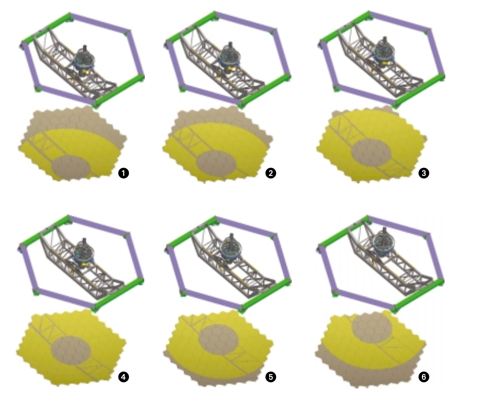
Figure A.1: When the tracker is centred (4), the telescope has its greatest light-collecting area, making it equivalent to a 9-m telescope. Even when the tracker is at its maximum off-axis position (1, 6), SALT is still equivalent to a 7-m telescope.
Figure A.2 shows the payload at the prime focus of the telescope without the tracker structure (cf. Fig. 2.2). The SAC is the grey cylinder at the bottom of the payload. At the top of the payload the RSS instrument with the camera is visible. Fig. A.3 shows a zoom-in with the covers removed: The slit-mask holder (green) and grating holder (yellow) are visible. The whole camera can rotate on the structure, depending on the articulation angle.
Figure A.4 shows the instruments underneath RSS: SALTICAM (orange), HRS fibre-feed (green, to the left of SALTICAM). The folding mirrors (grey with a red holder) are shown opposite SALTICAM, they direct the light coming from the SAC into the respective instrument. The SAC is shown underneath the instruments in green grid and yellow lens holder. Figure A.5 shows the SAC with blue ray tracing.
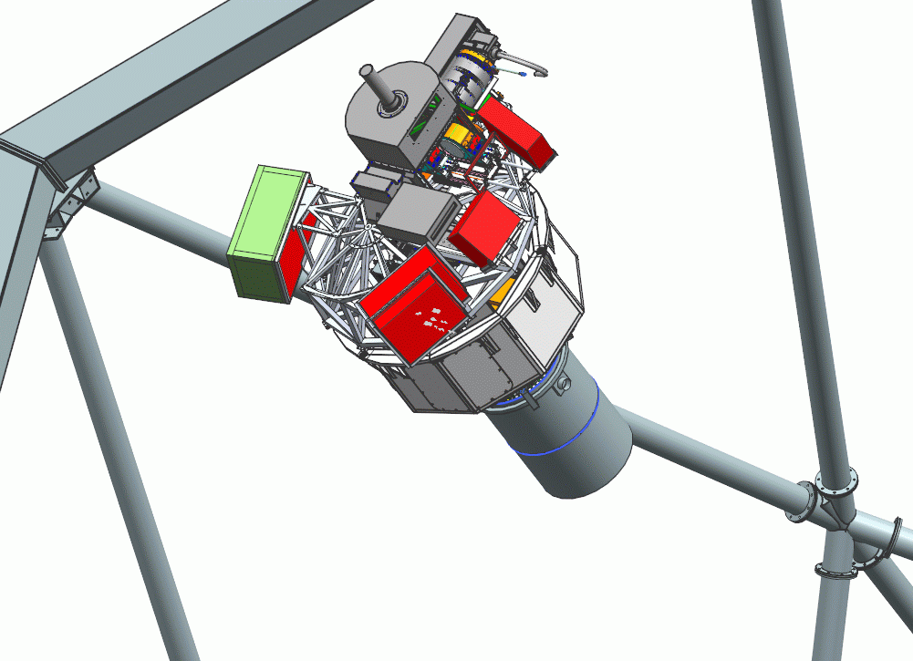
Figure A.2: The payload in the focal plane.

Figure A.3: The RSS instrument at the top of the payload.
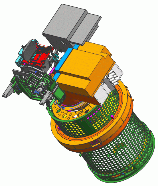
Figure A.4: SALTICAM (orange), HRS fibre-feed (green, to the left of SALTICAM). The folding mirrors (grey with a red holder) are opposite SALTICAM. The SAC is shown underneath the instruments in green grid and yellow lens holder.
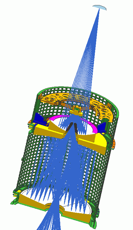
Figure A.5: SAC with ray tracing (blue) and focal plane indicated at the top.
A.5 SALTICAM Technical Information
Basic properties
Image Quality | See the SALTICAM optical design, Figure A.6. 0.3 arcsec (EE50), combined with SALT 0.6 arcsec (EE50), to give 0.67 arcsec image quality, independent of seeing. EE80 shall be no more than 0.5 arcsec. Distortion shall be less than 1 per cent. The mean plate scale shall be 107 micron/arcsec or 9.35 arcsec/mm within 1 percent. |
Science Field of View | 8 arcmin in diameter |
Guide Star Field of View | 10 arcmin in diameter |
Wavelength range | 320 – 950 nm |
Filters | 8 position filter unit. Available filters include U, B, V, R, I, clear; Sloan u', g', r', i', and z'; Strömgren u, v, b, y, H-beta wide, H-beta narrow, and red extensions SRE1, SRE2, SRE3, and SRE 4; H-alpha; neutral density; and short wavelength interference filters at 340 nm (FWHM 35 nm) and 380 nm (FWHM 40 nm). (see the PIPT for filter curves) |
CCD chips | E2V Technologies 44–82 |
Format | 2048 x 4102 x 15 micron square pixels per chip |
Plate scale | 0.14 arcsec/pixel |
Imaging area per chip | 30.7 x 61.5 mm2 imaging area per chip |
Readout capabilities | 2 readout amplifiers per chip |
Mosaicing | 2 x 1 mini-mosaic |
CTE | better than 99.99% |
Full well | 164 and 172 k e-/pix (for CCDs SALT-01 and SALT-02 respectively) |
Dark current | less than 1e-/pix/hr at 160 K |
Readout noise | less than 3.0 e-/pix at 100 kHz (10.0 usec/pix) (slow readout) |
CCD Controller | SDSU II (Leach) from Astronomical Research Camera Inc. |
Sensitivity | Thinned, back-illuminated. Deep depletion silicon. Astro Broad-Band anti-reflection coating. |
Observer specifics
NOTE: CCD-01 (aka CCD-B) is on the right side of the default SCAM display view and written SALTICAM files and CCD-02 (aka CCD-A) is on the left.
Quantum efficiency: | Delivered quantum efficiency for each chip is shown below: NOTE: CCD-01 (aka CCD-B) is on the right side of the scam view and written SCAM files and CCD-02 (aka CCD-A) is on the left.
| ||||||||||||||||||||||||||||||||||||||||||
Cosmetics: | Delivered cosmetics for each chip are shown below:
| ||||||||||||||||||||||||||||||||||||||||||
Gain: | Gain is user selectable and dependent on selected readout speed:
| ||||||||||||||||||||||||||||||||||||||||||
Pre-binning: | 1 x 1 to 9 x 9, independently in each direction | ||||||||||||||||||||||||||||||||||||||||||
Readout speed: | Frame transfer architecture: 0.10 sec frame transfer time 100–333 kHz (10–3.0 usec/pix). Observer specifies readout speed as "FAST" or "SLOW". | ||||||||||||||||||||||||||||||||||||||||||
Readout times: | Full frame, fast readout:
Full frame, slow readout:
See https://wiki.salt.ac.za/index.php/SCAM_overheads for details. | ||||||||||||||||||||||||||||||||||||||||||
Minimum exposure times: | The table shows the minimum exposure times for slot mode and frame transfer mode for all the valid binning parameters:
| ||||||||||||||||||||||||||||||||||||||||||
Windowing: | Up to 10 windows (prefer not to specify for P-V phase) | ||||||||||||||||||||||||||||||||||||||||||
Fastest windowed photometry: | 0.1 sec/sample with no dead time | ||||||||||||||||||||||||||||||||||||||||||
Count Rates: | Please use the most recent version of the SALTICAM simulator (http://astronomers.salt.ac.za/software/) for the most accurate exposure times and corresponding signal-to-noise ratios. |
Optical path and detectors
The lens system reduces the SALT f/4.2 prime focal ratio to f/2, thereby enabling the full 8-arcmin diameter science field of view, as well as almost all of the guide star field of view, to be captured on the 2x1 CCD mosaic. The lenses are made from UV-transmitting crystals, and the CCDs have excellent UV performance, so the instrument is expected to be very efficient at short wavelengths. The optical design is illustrated in Fig. A.6.
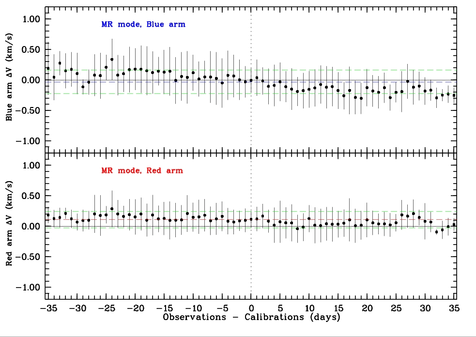
Figure A.6: SALTICAM optical path.
Figure A.7 shows the fields of view superimposed on the detector and includes:
- The edge of the science field of view (inner circle)
- The edge of the guide star field of view (outer circle)
- The two rectangular CCD chips separated by a 1.5 mm gap
- The (horizontal) frame transfer boundary
- The (vertical) boundary between the two halves on each chip read out by different readout amplifiers
Figure A.7: SALTICAM full layout.
The detector is a 2x2 mosaic of 2kx4kx15 micron pixel CCD 44–82 chips from E2V Technologies. These devices are thinned, back-illuminated and coated with the E2V Astro Broadband coating. They are also deep-depletion devices for better near-infrared sensitivity and lower fringing. A schematic of one of the chips is shown in Fig. A.8 (O'Donoghue et al 2004).
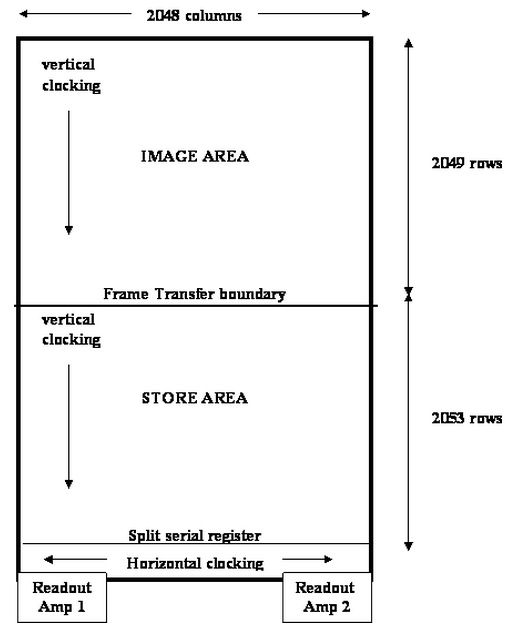
Figure A.8: SALTICAM schematic for one of the two CCDs.
High time-resolution modes: Frame Transfer and Slot mode
For moderate time resolution on the order of a few sec, Frame Transfer (FT) operation is used. This is explained by the left hand diagram in Fig. A.9: a mask (shown in grey) covers the lower half of each chip. At the end of each exposure, the image in the top half of the chip is rapidly (200 millisec) shifted to the lower half where it is readout while the next image in the top half accumulates during the next exposure.
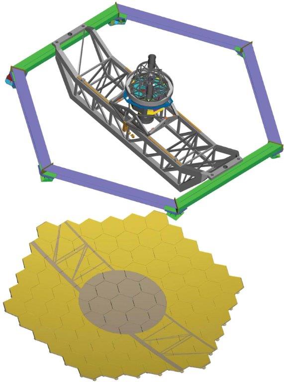
Figure A.9: SALTICAM schematic for frame transfer (left) and slot mode (right). The gray regions are masked.
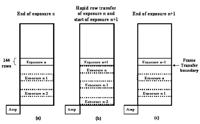
Figure A.10. SALTICAM schematic for slot mode readout.
Even faster sampling can be obtained with so-called slot mode: in this mode a mask is advanced over the entire chip except for a slot just above the frame transfer boundary. Instead of half frame transfers at the end of each exposure, 144 rows are moved and this allows exposure times as short as 100 millisec. The slot position is illustrated in the right hand diagram in Fig. A.9. Figure A.10 shows a schematic of the slot mode readout: Panel (a) shows the situation at the end of exposure n in one of the 4 amplifiers of the SALTICAM CCDs. The 144 rows indicated are transferred in about 15 millisec over the frame transfer boundary which is supposed to be aligned with the lower edge of the slot. At the end of this operation (Panel (b)), exposure n lies in the 144 rows below the FT boundary, and exposure n+1 begins. During exposure n+1, the 144 rows next to the readout register (indicated by exposure n-2 but in reality n-6) are read out, and the other data sections slowly scroll down by 144 rows. At the end of exposure n+1, the situation is then as in panel (c) which is the same layout as in panel (a) except that n is now replaced by n+1. See also O'Donoghue et al 2004.
Of course both FT mode and slot mode techniques require field of view to be sacrificed for time resolution: in FT mode, half the field of view is lost; in slot mode, only the slot is available for imaging. The intended use of slot mode is to position a rapidly varying target star and a brighter nearby companion star in the slot to perform differential photometry of the variable with respect to the comparison star. The telescope rho stage can be rotated to locate comparison stars at arbitrary position angles within the slot.
Optical efficiency
"Typical" instrument and system efficiencies are shown in Fig. A.11 and were calculated for the on-axis field position using:
- Optics:
- No absorption in any of the lens material or cryostat window (CaF2, BaF2, fused Si); Absorption by Sylgard 184 at two doublet interfaces;
- Reflection at 10 air-glass interfaces using the Spectrum Thin Films BBAR coating;
- Reflection at 2 air-glass interfaces using a single layer of MgF2 coating (see the 3310AE0001 Optical Design Issue 2.7.doc for details).
- The reflection or absorption in any filter is not included.
- CCDs: Quantum efficiency as delivered.
The SALTICAM efficiency (black line) is the product of the optics (blue) and the CCD (red) curves. For reference, RSS performance taken from Fig. 5 of the PFIS PDR Instrument Description Document is shown in green.
Figure A.12 shows the overall expected efficiency based on:
- Atmosphere (red): The standard atmospheric extinction curve for Sutherland at a zenith distance of 37 degrees.
- SALT + Fold (green dotted line): This is the minimum throughput taken from the system specification and includes reflectivity of the SALT Primary Mirror and the spherical aberration corrector (SAC), the SAC central obscuration, four per cent light losses at the four surfaces of the ADC, and the reflectivity of the fold mirror using the Livermore coating performance as supplied by David Buckley.
- Total (black): At the bottom is the product of the SALTICAM, Atmosphere and SALT+Fold curves.
See O'Donoghue et al 2003 for details.

Figure A.11: SALTICAM instrument efficiency with PFIS (now RSS) for comparison.
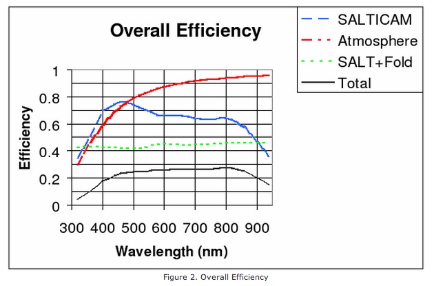
Figure A.12: SALTICAM overall efficiency (including telescope optics and atmosphere).
A.6 RSS Technical Information
See also http://www.sal.wisc.edu/PFIS/docs/rss-vis/ebb/pfis/observer/
RSS is an all-refractive collimator and camera system, optimised for spectroscopic performance in the 320-900 nm wavelength range. The collimator has 9 lenses in 5 groups plus a fold mirror before the last doublet. In the 150 mm diameter collimated beam are the shutter and the dispersers, which include one of six gratings (all volume phase holographic (VPH) gratings). The camera (F/2.2, 8.6 arcsec/mm) has 9 lenses in 4 groups, with the final lens, a field flattener, being the dewar window. All optical surfaces are spherical except for the first surface in the camera, which is an asphere.
The collimator is designed to work in the 320-1700 nm range, to accommodate a near-infrared camera; though the proposed NIR arm of RSS has subsequently been built as a separate instrument (NIRWALS). Air-glass interfaces in the collimator were coated with either a MgF2/Solgel hybrid or just a MgF2 anti-reflection coating. Camera surfaces were coated with a MgF2/Solgel hybrid or multi-layer anti-reflection coating.
To compensate for image error introduced by possible differences in filter thicknesses and uncompensated thermal effects, the camera has an active focus system. Focusing is accomplished by moving the singlet and the triplet in the camera together. Additionally, the camera needs to be refocused for each configuration, as the imaging was not optimised for all wavelengths simultaneously. However, a fixed focus position can be set for each configuration. Then final focus error due to filters/thermal effects can be removed.
Figure A.13 shows the main part of the RSS instrument and Fig. A.14 shows the optical path.
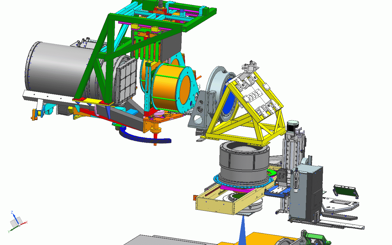
Figure A.13: RSS instrument. SALTICAM is located at the bottom of the image. Dark blue rays are shown being focused onto the first lens. The whole left hand section rotates on the dark blue track, depending on the articulation.
Figure A.14: RSS optics and optical path.
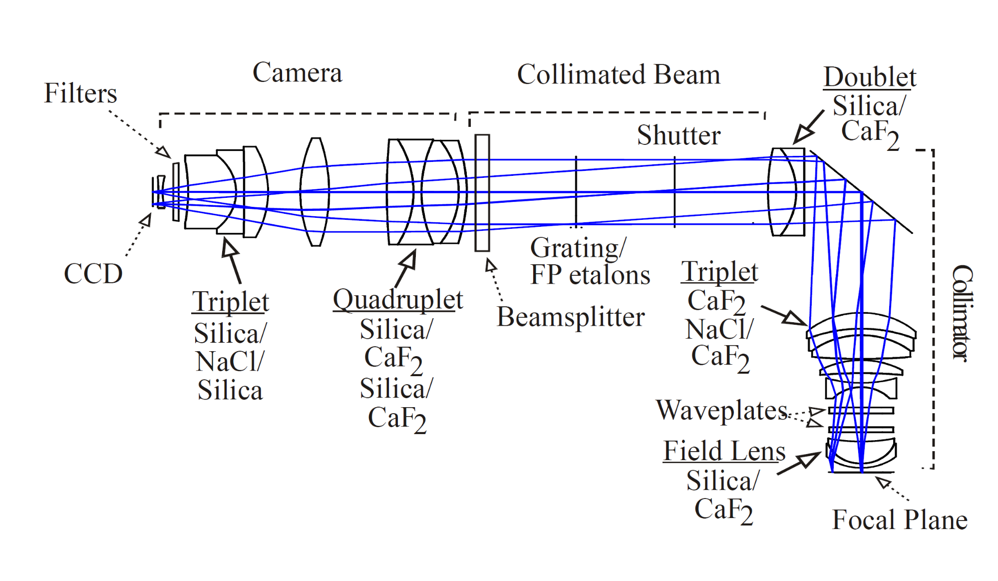
Detector (old & new)
This section has been updated with information for the new detector where it is currently known or estimated. Further clarifications will follow in due course.
The current (old) detector subsystem comprises a cryostat containing a 3x1 mini-mosaic of CCD chips. The chips are E2V (formerly Marconi) 44-82 CCDs with 2k x 4k x 15 micron pixels. The mosaic is housed in an evacuated cryostat and thermally connected to the cold end of a Cryotiger, which cools the chips sufficiently to render dark current insignificant while minimising QE reduction. The detectors are managed by an SDSU III CCD controller, which is in turn controlled by a PC. Figure A.15 shows the detector layout and the position of the slit. Readout speeds for various selected binnings and two readout modes are given in Table A.2. Note that horizontal and vertical binning result in different readout speeds, e.g., 2x1 (fast) takes 9.8 sec, while 1x2 (fast) takes 12.0 sec.
binning | Readout time `FAST’ mode (sec) | Readout time `SLOW’ mode (sec) |
1x1 | 17.8 | 46.0 |
2x2 | 6.6 | 12.6 |
4x4 | 3.3 | 5.0 |
6x6 | 2.2 | 3.2 |
8x8 | 1.6 | 2.2 |
9x9 | 1.8 | 1.5 |
2x1 | 9.8 | 22.8 |
4x1 | 5.1 | 11.3 |
6x1 | 3.7 | 7.7 |
8x1 | 3.1 | 6.5 |
| ||
1x2 | 12.3 | 26.0 |
1x4 | 9.7 | 17.0 |
1x6 | 9.3 | 14.0 |
1x8 | 8.8 | 12.0 |
Table A.2: Readout speeds for FAST and SLOW readout modes for the RSS.
Figure A.15: Old RSS detector system with slit position.
The new detector subsystem (expected October 2026) comprises a cryostat containing a single monolithic CCD chip. The chip is the E2V 231-C6 CCD with 6k x 6k x 15 micron pixels. The CCD is housed in an evacuated cryostat and thermally connected to the cold end of a Cryotiger, which cools the chip sufficiently to render dark current insignificant while minimising QE reduction. The detector is managed by an IUCAA CCD controller. Figure A.16 shows the detector layout relative to the old system.
Figure A.16: New RSS detector layout with the old 3-CCD system overlaid for reference.
Gratings
The VPH (volume phase holographic) gratings provide high diffractive efficiency and significantly reduced scattered light as compared to standard surface-relief gratings. Also, VPH gratings can be tuned to shift the diffraction efficiency peak to a desired wavelength. The use of such gratings requires the camera to be able to articulate, to accommodate various grating tilts. The grating resides on a rotatable stage, and the entire camera articulates about the same axis as the grating rotation.
Mechanical limitations require that the camera angle is quantized to every 0.75 degrees, with a maximum articulation of 100 degrees. Thus, a finite (but still large) number of camera positions are available. The camera angle determines the central wavelength on the detector, with longer wavelengths associated with larger camera articulation angles.
Filter transmission curves
The three UV filter transmission curves are shown in Fig. A.17 and the Blue filter transmission curves are shown in Fig. A.18.
Figure A.17: UV filter transmission curves. Only the filters UV-32 (PC03200), UV-34 (PC03400) and UV-38 (PC03850) are available.
Figure A.18: Transmission curve for Blue filter PC04600.
A.7 MOS System
RSS has multi-object spectroscopy capability. Slit-masks are fabricated using a laser cutting machine and inserted into a magazine that resides on the instrument. The magazine can carry 30 of these customised slitmasks at any given time. User designed slitmasks will be cut in Cape Town and stored on site with a unique barcode for identification.
One specific characteristic of VPH gratings to keep in mind is that the wavelength dependence of the efficiency depends on the input angle to the grating. In multi-object spectroscopy, the light entering through off-axis (in the dispersion direction) slits will hit the grating at different angles. Thus, the efficiency for the off-axis objects will be different than for the on-axis objects. This will in general not be symmetric either, i.e. objects that are at +2 arcminutes off-axis will have a different wavelength dependence of the efficiency from those at -2 arcminutes off-axis.
Additionally, the wavelength coverage on the detector for off-axis objects will be different than that for on-axis. So, the simultaneous wavelength coverage for a given grating setup with a multi-object slit mask will depend on how far off-axis the objects are.
Figures A.19 demonstrates these effects. The two plots show, for the PG3000 grating at 50 degrees grating angle, what the wavelength coverage and efficiency for the on-axis and two off-axis positions is. Note that for the full field (4 arcminutes off-axis) the simultaneous wavelength coverage is reduced and the efficiency can be as much as 50% lower for certain wavelengths.
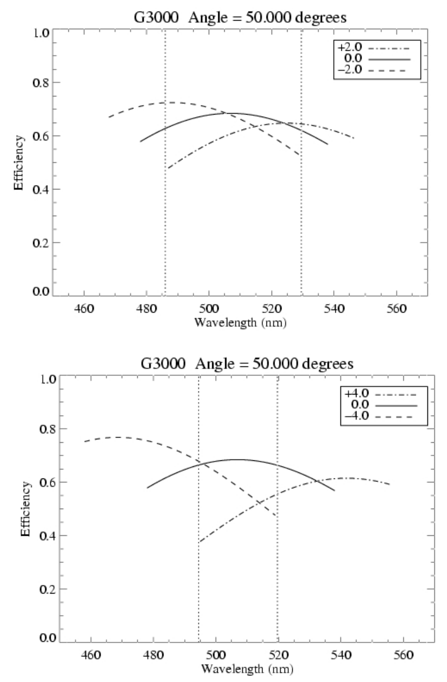
Figure A.19: Wavelength coverage and efficiency for the on-axis and two off-axis positions at +/- 2’(top panel) and +/- 4’ (bottom panel).
A.8 Narrow-band filter transmission curves
Please refer to Table 7.5 for the filter characteristics; the transmission curves are shown in Figure A.20.
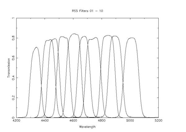
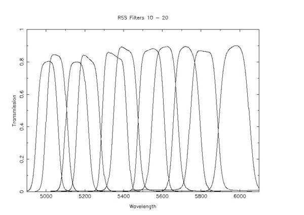
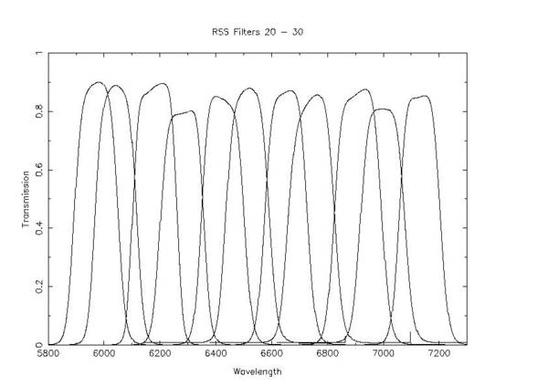
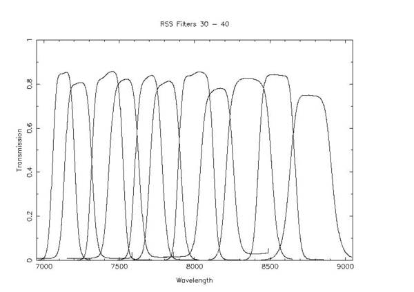
Figure A.20: Filter transmission curves for the FP narrow-band filters.
A.9 HRS Technical Information
The HRS is situated in an environmentally stable enclosure in the spectrograph room, underneath the telescope. Light is fibre-fed from prime focus (Fig. A.3; the green coloured instrument to the left of SALTICAM). The instrument’s optical path is shown in Fig. A.21.
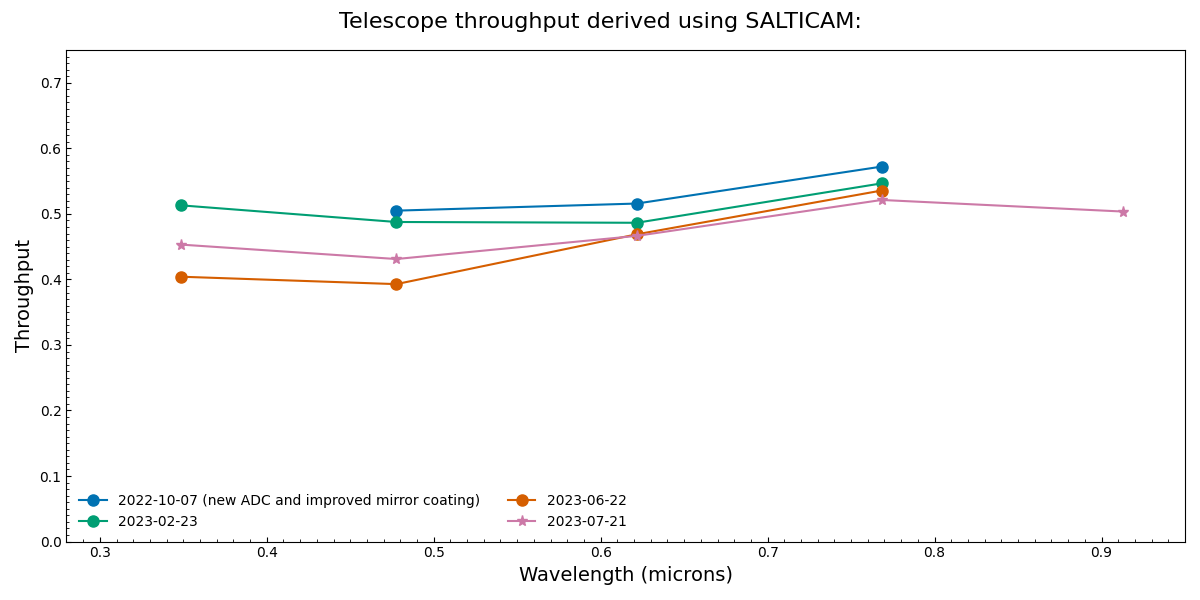
Figure A.21: Optical path for the HRS.
There are two cameras for the HRS, one for the blue arm (comprising 8 lenses and a clear aperture of 150mm), the other for the red arm (comprising 6 lenses and a clear aperture of 170mm). Both cameras have a cylindrical field flattening lens as the last element which has been made removable such that it can also act as the window for the detector cryostats.
The cameras were tested in double pass transmission (at 633nm) with an autocollimating flat mirror across the field of view of the cameras. Table A.4 gives the results. The wavefront error (WFE) for the cameras alone was found by subtracting the expected aberrations computed in Zemax from the measured performance.
Red camera: | |
Parameter | Measurement |
Focal length | 199.085mm |
WFE (on axis) | 0.27λ (λ=633nm) |
Global transmission | > 94.5% |
Blue camera: | |
Parameter | Measurement |
Focal length | 166.778mm |
WFE (on axis) | 0.44λ RMS (λ=633nm) |
Global transmission | > 85 % at 380nm > 88.5% at 410nm > 92% above 450nm |
Table A.3: Summary of camera tests
More details on the HRS can be found here:
SALT Proposal Info: 2026 Semester 2
[1] Grating used in off-Littrow configurations. Camera angles between 19.75 and 29.5 degrees
[2] Resolution estimated using Zemax model of the grating and a 1.5” slit